This guest post is by Karyn Meltz Steinberg on her preprint (with coauthors) Single haplotype assembly of the human genome from a hydatidiform mole, bioRxived here.

The human reference sequence is a mosaic of many DNA sources patched together to create the (mostly) contiguous chromosomes we all use every day in genomics labs. This mélange of haplotypes can result in reference representations that do not exist. For example, in GRCh37 at the MRC1 locus mixed haplotypes led to the presence of two gene models that represent false duplications and a gap that affected alignments of short reads. The problem of diploid source DNA was even worse in regions of structural variation where it was difficult to distinguish allelic variation from paralogous variation. The assembly structure in these regions was often wrong with either a collapsed assembly leading to missing sequence or with haplotype expanse, meaning 2, 3 or more haplotypes were represented on the chromosome sequence. The genomic resources associated with the essentially haploid complete hydatidiform mole, CHM1, have opened the door to allow us to address these issues.

What is essentially haploid? Well, what usually happens is that a sperm (usually bearing an X chromosome) fertilizes an egg that doesn’t have a nucleus (thus no DNA), the sperm DNA doubles, giving the correct chromosome complement, but with both pairs of chromosomes being identical. This cell divides and grows but does not form a normal embryo. In the early 1990s, Dr. Urvashi Surti was able to make an immortalized cell line from CHM1 tissue using hTERT. She karyotyped each passage to check that it maintained ploidy and that there were no gross somatic rearrangements.

Dr. Pieter de Jong then created an indexed BAC library from this high fidelity material. These BACs could then be used to resolve structurally complex regions such as 17q21.311. We continued working on sequencing more tiling paths across structurally complex regions; however, it was not practical or cost-efficient to Sanger sequence every single clone in the BAC library. As work continued, it became clear that developing the Primary Assembly using a single haplotype resource could be very powerful. This was possible due to the efforts of the Genome Reference Consortium (GRC) to extend the assembly model to include more than one sequence representation for a give region. We used Illumina sequencing technology and a reference based assembly algorithm developed at NCBI to produce an initial assembly. We then integrated the BAC sequences into the assembly to improve regions that are nearly impossible to assembly using whole genome strategies. The result is the highest quality whole genome sequence human genome assembly that is publicly available to date as assessed by metrics including contig and scaffold N50, repetitive element content and gene annotation.

So what–how can this help us, you ask? For the first time, one single haplotype of the human genome is represented. The fact that CHM1 is haploid means that we are able to finally go into the messy regions of the genome and resolve the genomic architecture as well as put any structural variation in the context of surrounding linked allelic variation. These are often biologically interesting regions; for example genes related to immune response and metabolism that are probably associated with complex traits are usually members of large gene families in segmentally duplicated sequence.

A fine example of the power of this haploid resource is also on BioRxiv, “Sequencing of the human IG light chain loci from a hydatidiform mole BAC library reveals locus-specific signatures of genetic diversity” (disclosure: this is also co-authored by me). The IG light chain genes encode for one part of immunoglobulin molecules that are expressed by B cells in response to antigenic stimulation (the heavy chain, IGH, was also resolved using CHM1 resources last year2). They are part of large gene families formed by duplication at three loci in the human genome. In previous versions of the reference assembly, these loci were comprised of sequence from multiple DNA sources that may have undergone somatic rearrangement. By sequencing BAC clones in a tiling path across these loci we now have a single haplotype representation of germline DNA sequence that allows us to perform accurate analyses of variation.

REFERENCES

1 Itsara, A. et al. Resolving the breakpoints of the 17q21.31 microdeletion syndrome with next-generation sequencing. American journal of human genetics 90, 599-613, doi:10.1016/j.ajhg.2012.02.013 (2012).
2 Watson, C. T. et al. Complete haplotype sequence of the human immunoglobulin heavy-chain variable, diversity, and joining genes and characterization of allelic and copy-number variation. American journal of human genetics 92, 530-546 (2013).

This post is by M.Mar Albà on her preprint (with co-authors) available from arRxiv Long non-coding RNAs as a source of new peptides.

Several recent studies based on deep sequencing of ribosome protected fragments have reported that many long non-coding RNAs (lncRNAs) associate with ribosomes (see for example Everything old is new again: (linc)RNAs make proteins! a comment by Stephen M Cohen). We have analyzed the original data from experiments performed in six different eukaryotic species and confirmed that this is a widespread phenomenon. This is paradoxical because lncRNAs apparently have very little coding capacity with only short open reading frames (ORFs) that do not show sequence similarity to known proteins.

In contrast to typical mRNAs, many lncRNAs are lineage-specific. Therefore, if they are translated, they should be similar to recently evolved protein-coding genes. This is exactly what we have found. It turns out that transcripts encoding young proteins show very similar properties to lncRNAs; short and non-conserved ORFs, low coding sequence potential, and relatively weak selective constraints.

Evidence has accumulated in recent years that new protein-coding genes are continuously evolving (The continuing evolution of genes by Carl Zimmer). The birth of a new functional protein is a process of trial and error that most likely requires the expression of many transcripts that will not survive the test of time. LncRNAs seem to fit the bill for this role.

This guest post is by Paul Bilinski on his paper with coauthors Diversity and evolution of centromere repeats in the maize genome BioRxived here.

Centromeres have the potential to play a central role in speciation, yet our ability to study them has been limited because of their repetitive nature. The centromeres of many eukaryotes consist partly of large arrays of short tandem repeats, though the actual sequence of the repeat varies widely across taxa. To investigate the whether the variation found in the tandem repeats themselves could inform our understanding of their evolutionary history we made use of the reference maize genome as well as resequencing data from several lines of maize and its wild relative teosinte.

Although tandem repeats should be identical upon duplication, our analysis of CentC in maize revealed that most copies genome-wide are unique. We observed only three instances where adjacent copies were identical in sequence and length, driving home the idea that these tandem repeats have accumulated immense diversity. Given such diversity, we wanted to investigate genetic relatedness across CentC copies.

Using positional and genetic relatedness information from the fully-sequenced centromeres 2 and 5, we found high within-cluster similarity, suggesting that tandem duplications drove most CentC copy number increase. Contrary to patterns seen in Arabidopsis (Kawabe and Nasuda 2005), principle coordinate analysis of repeats found no clustering by chromosome, with groups of CentC with similar sequence distributed across all of the chromosomes.

Another surprising discovery involved the origin of the biggest arrays of CentC. As an ancient tetraploid maize originally had 20 chromosomes with 20 centromeres. Processes of fractionation and rearrangement have led to the 10 chromosomes in the extant maize genome. Schnable et al (2011) were able to identify which chromosomal segments derive from each of maize’s ancient parents, referred to as subgenomes one and two. Wang and Bennetzen (2011) built on this information, and found that about half of the modern centromeres came from each parent. Inferring subgenome of origin by flanking regions, we found that all of the CentC clusters >20kb in length derive from subgenome 1. The proportions are less skewed when looking at clusters >10kb, though in all cases we see more bp of CentC assigned to subgenome 1 than we expect based on its total bp in the genome. This is particularly interesting because subgenome 1 also shows higher overall gene expression and fewer deletions than subgenome two (Schnable et al 2011).

The diversity of CentC seen might suggest that CentC repeats were reasonably static in the genome, persisting in the same spot for a long time with occasional increases in copy number via tandem duplication. However, fluorescent in situ hybridization suggested that domestication resulted in a large loss of CentC signal across many of maize’s 10 chromosomes. We confirmed and quantified the loss of CentC using resequencing data from a set of maize and teosinte lines (Chia et al. 2012).

Combined, our results suggest long term stability of CentC clusters with new copies arising from tandem duplication, while mutation serves to homogenize rather than separate clusters. We hope our insights into centromere repeat evolution will build toward a better understanding of their role in evolution.

This guest post is by Justin Blumenstiel on his preprint (with co-authors) When genomes collide: multiple modes of germline misregulation in a dysgenic syndrome of Drosophila virilis, available from bioRxiv here.

Does the activation of one transposable element (TE) family typically lead to the activation of many? If so, this would indicate a synergism between different TE families with significance for TE dynamics in natural populations. A standard model of TE dynamics typically takes into account population size, transposition rate (which may vary based on host defense) and selection against TE insertions. If the mobilization of one TE can lead to the mobilization of others, the transposition rate of one TE family could influence the transposition rate of others.

Hybrid dysgenic syndromes in Drosophila are an important model for TE dynamics when one TE family becomes mobilized. In the 1980’s, it was generally concluded that P element dysgenesis did not lead to mobilization of other TEs. However, studies in the D. virilis system of hybrid dysgenesis indicated otherwise. More recently, an analysis of transposition in the P element system indicated movement of elements other than the P element. Thus, it appears that co-mobilization may be a common feature of dysgenic syndromes.

What is the mechanism of co-mobilization? For the P element system, studies by William Theurkauf and colleagues point to the DNA damage response as key. Specifically, via Chk2 kinase, DNA damage signaling leads to perturbed piRNA biogenesis, which in turn leads to the activation of other elements under control of piRNA-based silencing. Does this mechanism also apply to other systems?

To study the mechanism of TE co-mobilization in the D. virilis system, we performed small RNA sequencing and mRNA sequencing experiments using germline material of reciprocal females of the dysgenic and non-dysgenic crosses. In contrast to the P element and I element systems, hybrid dysgenesis in D. virilis is more complex. For one, there is not a single element that has been proven to be the sole cause. This was previously shown, but in this study we identified several more elements that likely contribute. From small RNA sequencing, we find that TE mis-expression persists in the progeny of the dysgenic cross, without a persisting global defect in piRNA biogenesis. Rather, it appears that piRNA biogenesis defects are idiosyncratic across different TE families. Interestingly, we also find evidence that piRNA silencing loses specificity in the dysgenic cross, with some highly expressed genes becoming non-specific targets.

Overall, this study provided several insights, but the mechanism of co-mobilization in the D. virilis system remains unknown. The complexity of this syndrome makes it a challenge for study, but it may provide significant insight into genome dynamics of hybrids whose parents differ for more than one TE family. Future genetic analysis may allow us to determine the role of the DNA damage response in maintaining the activity of some TE families, but not others.

This guest post is by Radu Zabet on his preprint (with Boris Adryan) “Estimating transcription factor abundance and specificity from genome-wide binding profiles“, arXived here.

Binding of transcription factors (TFs) to the genome controls gene activity by either increasing or reducing the rate of transcription. We previously used stochastic simulations of the TF search mechanism (the facilitated diffusion mechanism which assumes both three-dimensional diffusion and one-dimensional random walk on the DNA) and investigated the binding of TFs to the genome; see http://www.plosone.org/article/info%3Adoi%2F10.1371%2Fjournal.pone.0073714#pone-0073714-g006 and http://nar.oxfordjournals.org/content/42/7/4196; also covered on https://haldanessieve.org/2013/04/09/our-paper-the-effects-of-transcription-factor-competition-on-gene-regulation/ and
https://haldanessieve.org/2014/01/10/author-post-physical-constraints-determine-the-logic-of-bacterial-promoter-architectures/. Our results confirmed that the binding profiles of TFs are mainly affected by the binding energy (usually represented by the Position Weight Matrix – PWM) between the TF and DNA and the number of molecules. What this means is that the binding profiles can now be approximated by the equilibrium occupancy and, thus, instead of running computationally expensive stochastic simulations, one can use the statistical thermodynamics framework to predict these binding profiles.

The statistical thermodynamics framework entails the computation of the statistical weight for each possible configuration of the system (the specific combination of locations on the DNA where TF molecules are bound). It immediately becomes clear that the number of possible configurations grows with increasing DNA segment size; thus making it impossible to compute genome-wide profiles. We addressed this using several approximations within the statistical thermodynamics framework and, based on these approximations, we derived an analytical solution. This allows the computation of genome-wide binding profiles by scanning the DNA quite similar to more naïve PWM based approaches. Our model takes as inputs four parameters: (i) the PWM scores, (ii) DNA accessibility data, (iii) the number of bound molecules and (iv) a factor that controls the specificity of the TF by rescaling the PWM scores. The first two are usually known from experimental data, while the last two are difficult to estimate from experiments and are usually computed by fitting the model to the data.

To test our model, we applied it to five ChIP-seq data sets (for Drosophila Bicoid, Caudal, Giant, Hunchback and Kruppel). Our results confirmed that, when including DNA accessibility data, the model fits the ChIP-seq profile with high accuracy (correlation coefficient > 0.65 for 4/5 TFs). Interestingly, we found that most TFs display lower abundance (in the range of 10-1000) than previously estimated (10000-100000). In addition, we also observed that while Bicoid and Caudal display high specificity (and our model predicts with good accuracy their ChIP-seq profiles), Giant, Hunchback and Kruppel display a lower specificity. Finally, we would like to emphasize that our method is applicable to any eukaryotic system for which the required data is available and can be applied genome-wide.

Our paper is accompanied by a how-to and all raw data to replicate our results: http://logic.sysbiol.cam.ac.uk/nrz/ChIPprofile/.

This guest post is by Olly Burren and Chris Wallace on their preprint, VSEAMS: A pipeline for variant set enrichment analysis using summary GWAS data identifies IKZF3, BATF and ESRRA as key transcription factors in type 1 diabetes, arXived here.

The idea for this paper came from reading a study by Liu et al. ( http://www.sciencedirect.com/science/article/pii/S0002929710003125) and the fact that summary p values from genome wide association studies are increasingly becoming publicly available. In the field of human disease, genome-wide association studies have been very successful in isolating regions of the genome that confer disease susceptibility. The next step however, is to understand mechanistically exactly how variation in these loci gives rise to this susceptibility. There are a myriad of pre-existing methods available for integrating genetic and genomic datasets, however things are complicated by the high degree of linkage disequilibrium that exists, which causes substantial inflation in the variance of any test statistic. This inter-SNP correlation must be taken into account, classically by permuting case/control status and recomputing association, requiring access to raw genotyping data. Indeed, this approach was taken in our previously published method see Heing et al. (http://www.nature.com/nature/journal/v467/n7314/full/nature09386.html) which uses a non-parametric test to compare distribution of GWAS p values from two sets of SNPs (“test” and “control”). As most researchers working with GWAS know gaining access to raw genotyping data is often difficult, and then how to include meta-analysis and imputed data? Liu et al., got around this by estimating the inter-SNP correlation using public datasets and sampling from a multivariate normal to generate simulated p values, analogous to the permuted p values possible with permuting phenotype status when raw data are available. VEGAS uses genotype data publicly available through the International HapMap project and aims to integrate GWAS results with trans eQTLs to identify causal disease genes.

Our thought was that by combining our previously published method, with the VEGAS approach, we could create a novel approach that would allow the integration of genetic information from GWAS with functional information from for example a set of micro-array experiments, crucially without the need for genotype information. The rationale being that it would help to prioritise future mechanistic studies, which can be costly and time-consuming to conduct. We also upped the stakes, and decided to use 1000 Genomes Project genotyping information for our estimations, to allow application to dense-genotyping technologies. The result was a software pipeline that takes as input a gene set of interest, a matched ‘control’ set and a summary set of GWAS statistics and computes an enrichment score.

Note that this approach differs from the Bayesian model suggested by Pickrell (https://haldanessieve.org/2013/12/16/author-post-joint-analysis-of-functional-genomic-data-and-genome-wide-association-studies-of-18-human-traits) as it focuses on comparing broad regions, rather than on considering more targeted genomic annotation, and in that sense is perhaps more akin to pathway analysis, although we do suggest that functionally defined genes sets, such as those found by knock down experiments in cell lines, may be more productive than using manually annotated pathways whose completeness can vary considerably.

To illustrate the method we applied it to a large meta-analysis GWAS study of type 1 diabetes (8000 case vs 8000 controls), and an interesting dataset examining the effect on gene-expression of knocking down a series of 59 transcription factors in a lymphoblastoid cell line see Cusanovich et al (http://www.plosgenetics.org/article/info%3Adoi%2F10.1371%2Fjournal.pgen.1004226). We identified three transcription factors, IKZF3, BATF and ESRRA, whose putative targets are significantly enriched for variation associated with type 1 diabetes susceptibility. IKZF3 overlaps a known type 1 diabetes susceptibility region, whereas BATF and ESRRA overlap other autoimmune susceptibility regions, validating our approach. Of course there are caveats interpreting results derived from cell lines, however we think it’s promising that our top hit lies in a region already associated with type 1 diabetes susceptibility.
Using the quantities already computed, once enrichment is detected, we implemented a simple technique to prioritise genes within the set. This allows the generation of a succinct list of genes that are responsible for the enrichment detected on the global level. Cross referenced with other information these can either be informative in their own right or be used to inform future studies.

This study is also an example of the preprint process speeding up scientific discovery. We knew about the Cusanovich dataset because they released a preprint on arXiv, which was caught by Haldane’s Sieve (https://haldanessieve.org/2013/10/22/the-functional-consequences-of-variation-in-transcription-factor-binding/) in October 2013. One email, and the authors kindly shared their complete results. Had we waited for it to be published in PLoS Genetics in March 2014, we’d have been five months behind where we are.

The major benefit is that all of the datasets employed are within the public domain. Our hope is that either this or other methods in the same vein will help to bridge the gap between GWAS and disease mechanisms, ultimately fuelling the development of new therapeutics.

This guest post is by Frank Albert and Leonid Kruglyak on their preprint (with co-authors) “Genetic influences on translation in yeast“.

This post is on a manuscript we recently posted to both biorXiv and arXiv on how genetic differences between yeast strains influence protein translation. Here, we give some background for the project and what the results mean in our eyes. We also highlight a few interesting aspects of regression analysis that may be useful to other researchers in genomics, but aren’t currently widely appreciated (at least they weren’t obvious to us before we dove into these data). We appreciate any comments and thoughts!

Protein translation and the genetics of gene expression

Our study was motivated by earlier reports that regulatory variation among individuals in a species can have surprisingly different effects on mRNA vs. on protein levels. For those not fully up to speed on these questions, here’s a quick recap. Individuals differ from each other in many aspects (e.g. in appearance and disease susceptibility), and for many traits, these differences are at least in part due to genetic variation. Research in genetics (both in humans and in other species) is focused on identifying DNA sequence variants in the genome that contribute to phenotypic variation, and on understanding the molecular mechanisms through which these variants alter traits. One general class of such mechanisms is alteration of gene expression, and genetic loci that affect gene expression are known as “expression quantitative trait loci” (eQTL). DNA sequence variants can change expression levels of genes in a number of ways, and some of the expression differences in turn are thought to alter organismal traits. Large and growing eQTL catalogues exist for several species. However, to measure “gene expression”, virtually all these studies measure mRNA rather than protein levels. This isn’t because mRNA is the more relevant molecule to look at, but primarily because mRNA is much easier and cheaper to measure on a global basis than are proteins. There have been a few studies in model organisms and—more recently— in humans that examined genetic variants that influence protein levels. Their results were surprising: the loci that influenced proteins (protein QTL, pQTL) were apparently often different from those that influenced mRNA levels, and vice versa. These results were both troubling and exciting. They were troubling because if genetic changes in protein levels are not a faithful reflection of effects on mRNA levels, the relevance of mRNA-based eQTL maps is less obvious. The results are exciting from a basic science perspective, because they suggest that lots of genetic variants that specifically influence posttranscriptional processes remain to be discovered.

Our current paper begins to explore these issues by measuring one such posttranscriptional process: protein translation, the process by which mRNA molecules are read by ribosomes and “translated” into peptide chains. Translation is interesting because there is literature that suggests that its regulation is a major determinant of protein levels, perhaps as important as the regulation of mRNA levels. Translation is also convenient because it is the last step along the gene expression cascade that can still be assayed using the high throughput sequencing technologies that underlie much of the current boom in genomics in general and eQTL detection in particular. The trick is to isolate only those bits of mRNA that sit inside of ribosomes as they march along the mRNAs during translation. These “ribosome footprints” can then be sequenced, counted, and compared to mRNA levels measured in parallel to get a quantitative readout of how much each gene is being translated.

For our current paper, we teamed up with Jonathan Weissman at UCSF. The Weissman lab pioneered measuring translation by sequencing, and Dale Muzzey (a postdoc with Jonathan) generated the data for our current experiment. We chose a very simple but powerful design: we compared translation in two strains of yeast that are genetically different from each other, and also measured allele-specific translation in the diploid hybrid between these two strains. Using the strain comparison, we can quantify the aggregate effect of all genetic differences between the two strains on translation. In the hybrid, we can specifically see the effects of those variants that act in cis, an important sub-group of eQTL.

We encourage you to read the detailed results in the paper, but in a nutshell, we found that genetic differences clearly do have an effect on translation—but not a terribly large one. Genes that differ in mRNA abundance typically also differ in footprint abundance, and the effect of translation was typically to subtly modulate mRNA differences, rather than erase them or create protein differences from scratch. While there are some exceptions, the take-home message is that on average, differences in protein synthesis are reasonably well approximated by differences in mRNA levels.

Thus, translation does not appear to create major discrepancies between eQTL and pQTL. So what explains such reported discrepancies? Without going into great detail, we think that at least a part of the explanation is that those discrepancies may have been overestimated. This fits with our recent paper in which we used extremely large yeast populations to map pQTL with higher statistical power, and recovered many pQTL at sites where earlier work had found an eQTL, but no pQTL. Are pQTL in most cases simply a reflection of eQTL? It is too early to tell, and we’ll need improved designs and datasets to answer to answer this question with certainty. At the very least, our recent work suggests that genetic influences on protein levels more accurately reflect those on mRNA levels than previous reports had suggested.

“Spurious” correlations and adventures in line fitting

While we worked on the translation paper, we encountered a few technical aspects that are worth sharing in some detail. Specifically, a natural question to ask is how differences in translation compare to differences in mRNA levels. When a gene differs in mRNA abundance between strains, does translation typically lead to a stronger or weaker footprint difference? Does translation typically “reinforce” or “buffer” mRNA differences (or is there no preference either way)? An intuitively attractive analysis is to plot the mRNA differences versus differences in “translation efficiency”, or TE (i.e. the amount of ribosome footprints divided by the amount of mRNA for a given gene). This comparison is shown in Figure 1 for our hybrid data.

In the figure, differences are plotted as log2-transformed fold changes so that zero indicates “no change”, and the resulting distributions of differences are more or less normally distributed. We see a seductively strong negative correlation between mRNA differences and TE differences. Taken at face value, this seems to suggest that mRNA differences are typically accompanied by a difference in TE that buffers the mRNA difference: more mRNA in one strain is counteracted by lower TE, presumably resulting in a protein difference that is smaller than the mRNA difference would predict.

However, this analysis is misleading. The key point is that the TE difference is not independent from the mRNA difference. In log2 space, the TE difference is simply the footprint difference minus the mRNA difference (in non-log space, the TE difference is the footprint difference divided by the mRNA difference). Therefore, the larger the mRNA difference becomes, the smaller the TE difference becomes simply by definition. The fact that the correlation between TE differences and mRNA differences is negative is by itself not informative about the relationship between differences in translation and mRNA levels. This can further be illustrated in Figure 2 (which is Supplementary Figure S4 in our preprint). Here, we simply draw two uncorrelated samples a and b from a normal distribution. The plot of b – a over a has a strong negative correlation, although there is no systematic relationship at all between these two quantities.

It turns out that the problems with comparing ratios (such as the TE difference) to their components (e.g., the mRNA difference, which serves as the denominator in computing TE) have been noted a long time ago (e.g., Karl Pearson termed them “spurious” correlations in 1897). They are worth remembering when carrying out functional genomic and systems biology data analyses in which multiple classes of molecules (mRNA, proteins, metabolites, etc.) are compared to each other and to ratios between them.

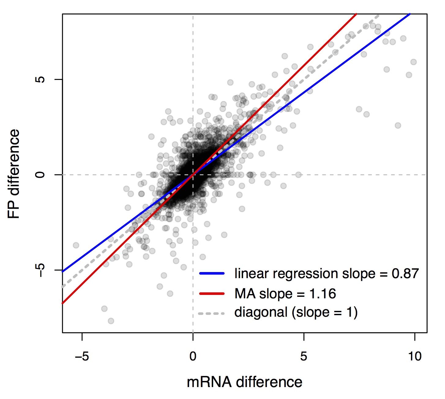
Because of this effect, we directly analyzed differences in the two quantities we measured: mRNA and ribosome footprint abundance. The slope of a linear regression between these two quantities was less than one (the blue line in Figure 3, which shows the data from the strain comparison). This might once again suggest a predominance of buffering interactions—for any given mRNA difference, we would predict a smaller footprint difference.

However, this inference is again misleading, because regression to the mean ensures that even if we measure the same quantity twice with some measurement noise (which is usually unavoidable), the slope of the regression line between these two replicates is always less than one. This is because when the first measure for a given gene is by chance larger than its true value, the measure is likely to be smaller in the second replicate. We estimated the regression slope between footprint differences and mRNA differences that would be expected if there were no preference for reinforcing or buffering interactions by using a randomization test that you can read about in the manuscript. The upshot is that the observed regression slope was steeper than those in the randomized data. We therefore concluded that on average, translation more often reinforces than buffers mRNA differences.

A related issue (pointed out to us by J.J. Emerson at UC Irvine) is that linear regression fits a line by minimizing only the error on the y-axis. This makes linear regression ideal for predicting y from x, but less than ideal for measuring the relationship (the slope) between x and y. For our purposes, it is better to use a different way of fitting lines to bivariate data: “Major Axis Estimation”. You can read all about MA in this great review, but briefly, the idea is to fit a line that minimizes the perpendicular distance of points from the line. The minimized error gets distributed between the y and the x axis, resulting in fitted lines that, unlike regression, provide unbiased estimates of the slope, and hence of the true linear relationship between x and y. Using MA on our data did not alter the conclusions we arrived at by using regression together with the randomization test, but it did provide more directly interpretable values for the various slopes. For example, the slopes in the randomized datasets were now centered on 1, whereas they had been degraded to be less than one using linear regression. The MA slope in our data was greater than one (the red line in Figure 3), supporting the inference of reinforcement.

These points on “spurious” correlations, regression to the mean and MA will be obvious to some (they were not to us going in), but we suspect and hope that they may prove useful for others working on genomic datasets.