This guest post is by Jerome Kelleher, on the preprint by Kelleher, Etheridge, and McVean titled “Efficient coalescent simulation and genealogical analysis for large sample sizes” available here from biorXiv.

In this post we summarise the main results of our recent bioRxiv preprint. We’ve left out a lot of important details here, but hopefully this summary will be enough to convince you that it’s worth reading the paper!

Coalescent simulation is a fundamental tool in modern population genetics, and a large number of packages exist to simulate various aspects of the model. The basic algorithm to simulate the coalescent with recombination was defined by Hudson in 1983, who also published the classical ms simulation program in 2002. Programs such as ms based on Hudson’s algorithm perform poorly for longer sequences, making simulation of chromosome sized regions under the influence of recombination impossible. The Sequentially Markov Coalescent (SMC) approximates the coalescent with recombination by assuming that each marginal genealogy depends only on its predecessor, making simulation much more efficient. The SMC can be a poor approximation when long range linkage information is important, however, and current simulations do not scale well in terms of sample size. Population-scale sequencing projects currently under way mean there is an urgent need for accurate simulations of hundreds of thousands of genomes.

We present a new formulation of Hudson’s simulation algorithm that solves these issues, making chromosome-scale simulation of the exact coalescent with recombination for hundreds of thousands of samples possible for the first time. Our approach begins by defining the genealogies that we are constructing in terms of integer vectors of a specific form, which we refer to as `sparse trees’. We generate recombination and common ancestor events in the same manner as the classical methods, but our approach to constructing marginal genealogies is quite different. When a coalescence within a marginal tree occurs, we store a tuple consisting of the left and right coordinates of the overlapping region, the parent and child nodes (which are integers), and the time at which the event occurred. We refer to these tuples as `coalescence records’, and they provide sufficient information to recover all genealogies after the simulation has completed. We implemented these ideas in a simulator called msprime, which we compared with the state of the art. For a fixed sample size of 1000 and increasing sequence length (with human-like recombination parameters), we found that msprime is much faster than comparable exact simulators and, surprisingly, is competitive with approximate SMC simulators. Even more surprisingly, we found that for a fixed sequence length of 50 megabases and increasing sample size, msprime was much faster than any existing simulator for large samples.

Storing the output of the simulations as coalescence records has major advantages. Because parent-child relationships shared by adjacent trees are stored only once, the correlation structure of the sequence of genealogies is explicit and the storage requirements minimised. To illustrate this, we ran a simulation of a 100 megabase chromosome with a roughly human recombination rate for a sample of 100,000 individuals. This simulation ran in about 6 minutes on a single CPU thread and used around 850MB of RAM. The resulting coalescence records required 88MB using msprime’s native HDF5 based storage format. Storing the same genealogies in Newick format requires around 3.5TB.

Highly compressed representations of data usually come at the cost of increased access time. In contrast, we can retrieve complete genealogical information from coalescence records many times faster than is possible using existing Newick-based methods. We provide a detailed listing of an algorithm to sequentially recover the marginal genealogies from a set of coalescence records and show that this algorithm requires constant time to transition between adjacent trees. This algorithm has been implemented as part of msprime’s Python API, and required around 3 seconds to iterate over all 1.1 million trees generated by the simulation above. We compared this performance to several popular tree processing libraries, and found that the fastest would require an estimated 38 days to parse the same set of trees in Newick format. Thus, in this example, by using msprime’s storage format and API we can store the same set of trees using around forty thousand times less space and parse them around a million times more quickly than Newick based methods.

We can also store mutational information in a natural and efficient way. If we have an infinite sites mutation that occurs on the parent branch of a particular node at a particular position on the sequence, then we simply store this (node, position) pair. This leads to a very compact representation of the combined genealogical and mutational state of a sample. We simulated 1.2 million infinite sites mutations on top of the genealogies generated earlier, which resulted in a 102MB HDF5 file containing the coalescence records and mutations. In contrast, the corresponding text haplotypes consumed 113GB of storage space. Associating mutations directly with tree nodes also allows us to perform some important calculations efficiently. We describe an efficient algorithm to count the total number of leaf nodes from a particular set below each node in the tree as we iterate over the sequence. This algorithm allows us to (for example) calculate allele frequencies within specific subsets in constant time. Many other applications of these techniques are possible.

The availability of faster and more accurate simulations may lead to interesting new applications, and so we conclude by discussing some potential applications of our work. Of particular interest is the possibility of inferring a set of coalescence records from real biological data, obtaining a compressed representation that can be efficiently processed. This is a very interesting and promising direction for future research.

This guest post is by Phillip Smith on his preprint Sex and Ageing: The Role of Sexual Recombination in Longevity

The two fold cost of sex is an old problem in the evolution of sex. Asexual organisms should out complete sexual organisms as they produce twice as many child bearing offspring as a sexual form. Some how sexual reproduction has pay for this twofold cost of sex.
Recombination has been shown in neutral network models to move the population toward the centre of genome space for protein models more efficiently than mutational load alone. This phenomenon of recombinational centring results in lower entropy and therefore greater robustness and stability. To investigate under which circumstances recombinational centring occurs we have to look at the relationship between genotype and phenotype. To do this we need some kind of machine that can simulate the complexity of a biology whilst being computation and conceptually simple enough to explore some of the parameter space of possible machines.
Biological entities must be some kind of complex machine. Machines can range in complexity from machines that do nothing (class I), through machines that oscillate (class II) to machines that are chaotic (class III). Somewhere on that continuum of machine types there are machines on the edge of chaos (class IV). For a cell to replicate a string (the genome) and a machine must interact to generate a new machine and a new string. In organism with sufficient genome length there is near zero probability that the parent and daughter cell have identical strings and machines. If the daughter cells string is incompatible with the machine then the cell will die.
Biology is an deeply nested system. Machines are made up of machines and the acceptability of a components state is dependent on the state of other machines within the nested hierarchy of the machine.
To capture the complexity of biology I developed these nested machines. They take a binary input string and use a machine to generate a smaller string representing the state of the machine at a higher level. The process is repeated at each stage until a single bit is left. If the bit is 1 then the string is accepted by the machine, else the string is rejected. To keep the parameter space small the wolfram elemental cellular automata ECA were used as the machines. The same machine was used for each level. There are 256 machines and they are known to have machines in all four wolfram classes. Rule 30 is a pseudo-random number generator for long strings (100) bits. Rule 110 is a turing complete machine capable of computation.
Movement of the population towards the centre of the genome space reduces mutational load this was shown to be very pronounced in the class IV machines whereas in the class III chaotic machines the opposite was observed, recombination increased mutational load. This shows that recombinational centring requires class IV machines to work, these are the same machines that are thought to me most similar to the complexity found in biology and the most likely to capable of computation.
Obviously the less entropy and individual starts with the longer they will be able to accumulate disorder and will be both more mutationally robust and robust to unpredicted environmental insult.
It is therefore reasonable that they should live longer. This was tested by simulating ageing on populations of differing machines at asexual and sexual equilibrium. Essential ageing was considered a random walk in genome space. The closer you start to the well connected centre the longer you will survive. Class IV machines saw the best increase in resistance to ageing.
For Rule 110 it was shown that this resistance to ageing was sufficient to compensate for the twofold cost of sex if the age of maturation was late enough in the lifespan as sexual forms had greater reproductive potential.
It is suggested that the increased resistance to ageing is sufficient to compensate for the twofold cost of sex in large complex organisms.

This guest post is by Benjamin Peter on his preprint Trees, Population Structure, F-statistics!

I began thinking about this paper more than a year ago, when Joe Pickrell and David Reich posted their perspective paper on human genetic history on biorxiv. In that paper, they presented a very critical perspective of the serial founder model, the model I happened to be working on at the time. Needless to say, my perspective on the use (and usefulness) of the model was, and still is, quite different.

Part of their argument was based on the usage of the F3-statistic, and the fact that it is negative for many human populations, indicating admixture. Now, at that time, I was familiar with the basic idea of the statistic and had convinced myself – following the algebraic argument in Patterson et al. (2012) – that it should be positive under models of no admixture. However, I still had many open questions that this paper did not answer. Why should we use F2 as a measure of genetic drift to begin with? Why does F3 have this positivity property? How robust is this to other structure models? The ‘path’-diagrams that Patterson et al. (2012) used personally did not help me, because I am not familiar with Feynman diagrams, and I did not understand how drift could have ‘opposite’ directions.

The other primary sources did not help me, partly because they are buried in supplements and repetitive. Unfortunately, I initially missed what I now find the most comprehensive resource – the Supplementary Material of Reich et al. (2009), which did not help my understanding. However at that time – early summer last year – I had a thesis to finish, and so the F-statistics left my mind.

I finished my Ph. D. in July, moved to Chicago in October 2014 and forgot about F-statistics in the meantime. When I started my postdoc, John Novembre proposed that I have a look at EEMS, a program one of Matthew’s former students, Desi Petkova, had developed to visualize migration patterns. Strikingly, Desi also used a matrix of squared difference in allele frequency, but she did so in a coalescence framework and for diploid samples, as opposed to the diffusion framework and population sample used for the F-statistics. However, the connection is immediately obvious, and it took only a few pages of algebra to figure out what is now Equation 5 in the paper; namely that F2 has a very easy interpretation under the coalescent.

This was a very useful result, and was what eventually made me decide to start writing a paper, and research the other issues I did not understand about F-statistics. It takes very little algebra (or some digging through supplementary materials) to figure out that F3 and F4 can be written in terms of F2. The interesting bit, however, is the form of these expressions – they immediately reminded me of quantities that are used in distance-based phylogenetics – the Gromov product and tree splits, and made it obvious, that the statistics should be interpreted in that context as tests of treeness, with admixture as the alternative model, and that F3 and F4 are just lengths of external and internal branches on a tree, and that the workings of the tests can be neatly explained using that phylogenetic theory.

Now, essentially a year later, I finished a version of my paper that I am comfortable with sharing. Because of my initial difficulties with the subject – and my suspicion I might not be the only one that only has a vague understanding of the statistics – I kept the first part as basic as possible, starting with how drift is measured as decay in heterozygosity, as increase in uncertainty or relatedness, then explore in depth the phylogenetic theory underlying the null model of the admixture tests, and briefly talk about the path interpretation of the admixture model. Only then I present my main result, the interpretation in terms of coalescent times and internal branch lengths, some small simulations as sanity checks and some applications and population structure models.

A big challenge has been to attribute ideas correctly, sometimes because sources were sometimes difficult to find, and sometimes because key ideas were only implicitly stated. So if parts are unclear, or if I misattributed anything, please let me know, and I am happy to fix it. Similarly, if there are parts of the manuscript that are hard to understand, please contact me, the aim of this paper is meant to serve both as an useful introduction to the topic, and to present some interesting results.

This guest post is by William DeWitt on his preprint (with co-authors) “Immunosequencing reveals diagnostic signatures of chronic viral infection in T cell memory”.

This is a post about our preprint at biorXiv. Although it’s a paper on infectious disease and immunology, our colleague (and Haldane’s Sieve contributor) Bryan Howie suggested we might engage the community here, since we think there are interesting connections to standard GWAS methodology. I’ll start with a one-paragraph immunology primer, then summarize what we’ve been up to, and what’s next.

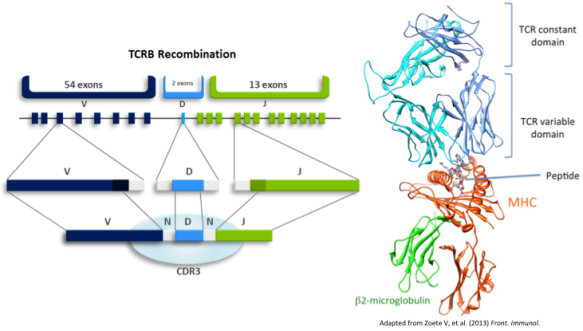
Cell-mediated adaptive immunity is effected by T cells, which recognize infection through interface of the T cell receptor (TCR) with foreign peptides presented on the surface of all nucleated cells by major histocompatibility complex (MHC). During development in the thymus, maturing T cells somatically generate genes encoding the TCR according to a random process of V(D)J recombination and are passed through selective barriers against weak MHC affinity (positive selection) and strong self-peptide affinity (negative selection). This results in a diverse repertoire of self-tolerant receptors from which to deploy specific responses to threats from a protean universe of evolving pathogens. Upon recognition of foreign antigen, a T cell proliferates, generating a subpopulation with identical-by-descent TCRs. This clonal selection mechanism of immunological memory implies that the TCR repertoire dynamically encodes an individual’s pathogen exposure history, and suggests that infection with a given pathogen could be recognized by identifying concomitant TCRs.

In this study, we identify signatures of viral infection in the TCR repertoire. With a cohort of 640 subjects, we performed high-throughput immunosequencing of rearranged TCR genes, and serostatus tests for cytomegalovirus (CMV) infection. We used an analysis approach similar to GWAS; among the ~85 million unique TCRs in these data, we tested for enrichment of specific TCRs among CMV seropositive subjects, identifying a set of CMV-associated TCRs. These were reduced to a single dimension by defining the pathogen memory burden as the fraction of an individual’s TCRs that are CMV-associated, revealing a powerful discriminator. A binary classifier trained against this quantity demonstrated high cross validation accuracy.

The binding of TCR to antigen is mediated by MHC, which is encoded by the highly polymorphic HLA loci. Thus, the affinity of a given TCR for a given antigen is modulated by HLA haplotype. HLA typing was performed for this cohort according to standard methods, and we investigated enrichment of specific HLA alleles among the subjects in which each CMV-associated TCR appeared. Most CMV-associated TCRs were found to have HLA restrictions, and none were associated with more than one allele in any locus.

There is substantial literature identifying TCRs that bind CMV antigen through low-throughput in vitro methods, including so-called public TCRs, which arise in many individuals. Most public CMV TCRs were present in our data, however most were not in our list of diagnostically useful CMV-associated TCRs. This is understood by considering that V(D)J recombination produces different TCRs with different probability. Public TCRs, having high recombination probability, will be repeatedly recombined in the repertoires of all subjects, regardless of CMV infection status; their presence is not diagnostic for CMV serostatus, even if they are CMV-avid. Conversely, CMV-avid TCRs with low recombination probability will be private to one subject (if present at all) in any cohort of reasonable size; their enrichment in CMV seropositive subjects is not detectable. CMV-avid TCRs with intermediate recombination probability recombine intermittently, residing transiently in the repertoires CMV naïve individuals and reliably proliferating upon CMV exposure; the presence of these TCRs in an immunosequencing sample is diagnostic for infection status.

It may be interesting to draw a comparison with GWAS, where selection drives disease-associated variants with high effect size to low population frequency, out of reach of the detection power of any study. In contrast, the V(D)J recombination machinery is constant across individuals, and CMV-avid TCRs appear to span a broad range of recombination probabilities from public to private. This includes plenty in an intermediate regime of what we might call diagnostic TCRs, which can be used to build powerful classifiers of disease status that aren’t blunted by suppression of the most relevant features.

We’ll be making the data from this study available online, constituting the largest publically accessible TCR immunosequencing data set. It’ll be fun to see what other groups do with it.

Some things we’re still working on:
• We did cross validation to assess diagnostic accuracy (yellow curve in the ROC figure), including recomputation of CMV-associated TCRs for each holdout. Results are encouraging, but a more convincing test will be to diagnose a separate cohort. We’re in the process of acquiring these data.
• MHC polymorphism suggests that thymic selection barriers censor different TCRs in individuals with different HLA haplotype. We’ve done preliminary work identifying TCRs that are associated with more common HLA alleles, indicating the possibility of HLA typing from immunosequencing data. Interestingly, this necessitates a two-tailed test due to modulation of both positive and negative selection.
• Our association analysis relies on the recurrence of TCRs with identical amino acid sequence across individuals, but we’d like to be able to define TCR motifs more loosely, so that we can detect enrichment without requiring identity. This necessitates a similarity metric in amino acid space that captures similarity in avidity. We have some ideas here, and are testing them out on some validation data. It’s definitely a tough one, but could substantially increase power in this sort of study.

This guest post is by Matthew Hartfield (@mathyhartfield) on his preprint (with Sylvain Glemin) “Limits to adaptation in partially selfing species”, available from bioRxiv here

Our paper “Limits to adaptation in partially selfing species” is now available from bioRxiv. This preprint is the result from a collaboration that has been sent back-and-forth across the Atlantic for well over a year, so we are pleased to see it online.

Haldane’s Sieve, after which this blog is named, is a theory pertaining to the role of dominance in adaptation, which was initially developed for outcrossing species and then shown to be absent in selfing species. When beneficial alleles initially appear in diploid individuals, they do so in heterozygote form (so only one of two alleles at the locus carry the advantageous type). Mathematically, these mutations have selective advantage 1 + hs where h is the degree of dominance, and s the selective advantage. Haldane’s Sieve states that recessive mutations (h 1/2), because selection is not efficient on heterozygotes if mutations are recessive. However, self-fertilising individuals are able to rapidly create homozygote forms of the mutant, increasing the efficacy of selection acting on them. Yet selfing also increases genetic drift, and hence the risk that these adaptations will go extinct by chance. Consequently, an extension of Haldane’s Sieve states that if the mutation is recessive (h 1/2).

This result holds for a single mutant in isolation. Yet mutants seldom act independently; they usually arise alongside other alleles in the genome, each of which has their own evolutionary outcomes. A known additional advantage of outcrossing is that, through recombining genomes from each parent, selected alleles can be moved from disadvantageous genomes to fitter backgrounds. For example, say an adaptive allele was present in a population, and a second adaptation arose at a nearby locus. If the second allele was not as strongly selected as the first, then it has to arise on the same genome as the initial adaptation. Otherwise it is likely to be lost as the less-fit genotype is replaced over time, a process known as selective interference. However, outcrossing can unite the two mutations into the same genome, so both can spread.

Despite these potential advantages of outcrossing, the effect of selective interference has not yet been investigated in the context of how facultative selfing influences the fixation of multiple beneficial alleles. Our model therefore aimed to determine how likely it is that secondary beneficial alleles can fix in the population, given an existing adaptation was already present, and reproduction involved a certain degree of self-fertilisation.

After working through the calculations, two subtle yet important twists on Haldane’s Sieve revealed themselves. First, due to the effects of selection interference, Haldane’s Sieve is likely to be reinforced in areas of low recombination. That is, recessive mutants are more likely to be lost in outcrossers (when compared to single-locus results), with similar losses for dominant mutations in self-fertilising organisms. Secondly, we also investigated a case where the second beneficial mutant could be reintroduced by recurrent mutation. In this case, selection interference can be very severe in selfers due to the lack of recombination. Hence some degree of outcrossing would be optimal to prevent these beneficial alleles from being repeatedly lost, even if they are recessive. In the most extreme case, complete outcrossing is best if secondary mutations only confer minor advantages.

In recent years, the role that selection interference plays in affecting mating system evolution is starting to become recognised. Our theoretical study is just one of many that elucidates how important outcrossing can be in augmenting the efficacy of selection. Our hope is that these studies will spur on further empirical work quantifying the rate of adaptation in species with different mating systems, to further unravel why species reproduce in vastly different ways.

This guest post is by David Castellano and Adam Eyre-Walker on their preprint (with co-authors) Adaptive evolution is substantially impeded by Hill-Robertson interference in Drosophila.

Our paper “Adaptive evolution is substantially impeded by Hill-Robertson interference in Drosophila”, in which we investigate the role of both the rate of recombination and the mutation rate on the rate of adaptive amino acid substitutions, has been available at biorxiv (http://dx.doi.org/10.1101/021600) since 27 June.

Population genetics theory predicts that the rate of adaptive evolution should depend upon the rate of recombination; genes with low rates of recombination will suffer from Hill-Robertson interference (HRi) in which selected mutations interfere with each other (see the figure below): a newly arising advantageous mutation may find itself in competition for fixation with another advantageous mutation at a linked locus on another chromosome in the population, or in linkage disequilibrium with deleterious mutations, which will reduce its probability of fixation if it can not recombine away from them.

A schematic HRi example among adaptive alleles (left) and among adaptive and deleterious alleles (right).

Likewise, it is expected that genes with higher mutation rates will undergo more adaptive evolution than genes with low mutation rates. More interestingly an interaction between the rate of recombination and the rate of mutation is also expected; HRi should be more prevalent in genes with high mutation rates and low rates of recombination. No attempt has been done so far to quantify the overall impact of HRi on the rate of adaptive evolution for any given genome. In our paper we propose a way to quantify the number of adaptive substitutions lost due to HRi – approximately 27% of all adaptive mutations, which would go to fixation since the split of D. melanogaster – D. yakuba if there was free recombination, are lost due to HRi. Moreover, we are able to estimate how the fraction of lost adaptive amino acid substitutions to HRi depends on gene’s mutation rate. In agreement with our expectations, genes with high mutation rates lose a significantly higher proportion of adaptive substitutions than genes with low mutation rates (43% vs 11%, respectively).

An open question is to what extent HRi affects rates of adaptive evolution in other species. Moreover, the loss of adaptive substitutions to HRi can potentially tell us something important about the strength of selection acting on some advantageous mutations, since weakly selected mutations are those that are most likely to be affected by HRi. This will require further analysis and population genetic modeling, but in combination with other sources of information, for example, the dip in diversity around non-synonymous substitutions, the site frequency spectrum the high frequency variants that are left by selective sweeps it may be possible to infer much more about the DFE of advantageous mutations than previously thought.

It will be of great interest to do similar analyses to those performed here in other species.

Comments very welcome!
David and Adam

This guest post is by Matthew Hartfield (@mathyhartfield) on “Coalescent times and patterns of genetic diversity in species with facultative sex”.

Our paper “Coalescent times and patterns of genetic diversity in species with facultative sex”, in which we investigate the genealogies of facultative sexuals, is now available from the biorxiv.

Most evolutionary biologists are obsessed with sex. Explaining why organisms reproduce sexually by combining genetic material is a tough problem. The main issue lies with the fact that asexuality (reproduction via clonality) should be able to outcompete sexuals due to sheer weight of numbers. Various theories have been put forward to explain why sex is so widespread. The majority of these revolve around the idea that exchanging genetic material enables the fittest possible genotype to be created, while that of asexuals should degrade over time.

While such theories are ubiquitous, data to test them has been scarce. Recent years have seen a boom in exploring the evolution of sex experimentally using facultative sexual organisms: species that can switch between sexual and asexual reproduction. Such experiments have demonstrated how sexual reproduction can evolve when exposed to stressful environments, or when moving between environmentally different areas. Yet major questions remain regarding what the underlying genetic causes of these transitions are. In addition, there are plenty of organisms that undergo ‘cryptic’ sex, which cannot be observed directly but can with genomic sequence analyses.

Coalescent models are important for analysing genomic data. These tools determine the relationship between neutral markers, and hence make predictions on how genetic diversity is affected depending on environmental structuring, localised natural selection, or other effects. However, classic models cannot be applied to systems with partial asexuality, as they assume the population reproduces entirely sexually.

We worked on introducing partial rates of sex into these models. In the simplest case (one population with a fixed rate of sex), we recovered a classic prediction that extensive divergence between alleles at the same site arises. This phenomenon occurs since lack of sex keeps the two alleles distinct over evolutionary time; only a rare bout of sex has any chance of creating the segregation needed for them to be descended from the same allele.

A schematic of Allelic Sequence Divergence (ASD) in asexuals: Xs are distinct mutations at each neutral site.

After recovering this familiar result, we worked to extend coalescent theory in partial asexuals to include various other biological phenomena. Two effects we looked at were gene conversion, and heterogeneity in sex rates that change over time or space.

Gene conversion, where one DNA sequence replaces part of a homologous chromosome, is usually regarded as being of minor evolutionary importance. Yet numerous studies of facultative sexuals often observe it as a common force, especially in species not exhibiting allelic sequence divergence (ASD). Could the two be related? Excitingly, we found that low rates of gene conversion become important in organisms with low rates of sex. That is, once sex becomes so rare as to caused ASD, small rates of gene conversion can then reverse the process, homogenizing alleles again. Rather than having higher diversity than otherwise similar sexual populations as expected with ASD (in the absence of gene conversion), asexual populations will have less diversity than comparable sexual populations if gene conversion is not too low.

It is also known that many organisms change their rates of sex over time or location, which can be triggered by environmental cues or organismal stress. By investigating such variation in the rate of sex, the analysis elegantly shows how even a short burst to obligate sex (over tens of generations) is enough to jumble genomes in the population, hence giving the same outcome as long-term obligate sex. If rates of sex are also different in separate geographical locals, then these differences can be detected if there is little gene flow between regions. Otherwise, both areas display intermediate rates of sex.

Coalescent tools are popular since they can be used to simulate complex evolutionary outcomes, which are then tested against genomic data. We used the mathematical analyses to outline a coalescent algorithm to account for partial rates of sex, and predict genetic diversity, under numerous scenarios. The code is available online (http://github.com/MattHartfield/FacSexCoalescent) for others to use.

These are exciting times for population genetics and evolution, with cheaper sequencing costs making it possible to wade through the genomes of more individuals than before. Yet accurately exploring the genetic landscape requires the creation of mathematical tools that accounts for organismal life history. These results will provide the first of many buildings blocks to determine the effects of selection and the environment on the evolution of facultative sexuals. They might eventually reveal why sex is so prevalent in nature.

This guest post is by William Wen on his preprint “Bayesian Model Comparison in Genetic Association Analysis: Linear Mixed Modeling and SNP Set Testing”, arXived here.

Our paper “Bayesian Model Comparison in Genetic Association Analysis: Linear Mixed Modeling and SNP Set Testing” has been published in the journal Biostatistics, the preprint is also updated on the arXiv. The paper discusses linear mixed models (LMM) and the models commonly used for (rare variants) SNP set testing in a unified Bayesian framework, where fixed and random effects are naturally treated as corresponding prior distributions. Based on this general Bayesian representation, we derive Bayes factors as our primary inference device and demonstrate their usage in solving problems of hypothesis testing (e.g., single SNP and SNP set testing) and variable selection (e.g., multiple SNP analysis) in genetic association analysis. Here, we take the opportunity to summarize our main findings for a general audience.

Agreement with Frequentist Inference

We are able to derive various forms of analytic approximations of the Bayes factor based on the unified Bayesian model, and we find that these analytic approximations are connected to the commonly used frequentist test statistics, namely the Wald statistic, score statistic in LMM and the variance component score statistic in SNP set testing.

In the case of LMM-based single SNP testing, we find that under a specific prior specification of genetic effects, the approximate Bayes factors become monotonic transformations of the Wald or score test statistics (hence their corresponding p-values) obtained from LMM. This connection is very similar to what is reported by Wakefield (2008) in the context of simple logistic regression. It should be noted the specific prior specification (following Wakefield (2008), we call it implicit p-value prior) essentially assumes a larger a priori effect for SNPs that are less informative (either due to a smaller sample size or minor allele frequency). Although, from the Bayesian point of view, there seems to be a lack of proper justification for such prior assumptions in general, we often note that the overall effect of the implicit p-value prior on the final inference may be negligible in practice, especially when the sample size is large (We demonstrate this point with numerical experiments in the paper).

For SNP set testing, we show that the variance component score statistic in the popular SKAT model (Wu et al. (2011)) is also monotonic to the approximate Bayes factor in our unified model if the prior effect size under the alternative scenario is assumed small. Interestingly, such prior assumption represents a “local” alternative scenario for which score tests are known to be most powerful.

The above connections are well expected: after all, the frequentist models and the Bayesian representation share the exact same likelihood functions. From the Bayesian point of view, the connections reveal the implicit prior assumptions in the Frequentist inference. These connections also provide a principled way to “translate” the relevant frequentist statistics/p-values into Bayes factors for fine mapping analysis using Bayesian hierarchical models as demonstrated by Maller et al. (2012) and Pickrell (2014).

Advantages of Bayesian Inference

Bayesian Model Averaging

Bayesian model averaging allows simultaneous modeling of multiple alternative scenarios which may not be nested or compatible with each other. One interesting example is in the application of rare variants SNP set testing, where two primary classes of competing models, burden model (assuming most rare causal variants in a SNP set are either consistently deleterious or consistently protective) and SKAT model (assuming the rare causal variants in a SNP set can have bi-directional effects), target complimentary alternative scenarios. In our Bayesian framework, we show that these two types of alternative models correspond to different prior specifications, and a Bayes factor jointly considering the two types of models can be trivially computed by model averaging. A frequentist approach, SKAT-O, proposed by Lee et al. (2012) achieves the similar goal by using a mixture kernel (or prior from the Bayesian perspective). We discuss the subtle theoretical difference between the Bayesian model averaging and the use of SKAT-O prior and show by simulations, the two approaches have similar performance. Moreover, we find that the Bayesian model averaging is more general and flexible. To this end, we demonstrate a Bayesian SNP set testing example where three categories of alternative scenarios are jointly considered: in addition to the two aforementioned rare SNP association models, a common SNP association model is also included for averaging. Such application can be useful for eQTL studies to identify genes harboring cis-eQTLs.

Prior Specification for Genetic Effects

The explicit specification of the prior distributions on genetic effects for alternative models is seemingly a distinct feature of Bayesian inference. However, as we have shown, even the most commonly applied frequentist test statistics can be viewed as resulting from some implicit Bayesian priors. Therefore, it is only natural to regard the prior specification as an integrative component in modeling alternative scenarios. Many authors have shown that it is effective to incorporate functional annotations into genetic association analysis through prior specifications. In addition, we also show that in many practical settings, the desired priors can be sufficiently “learned” from data facilitated by Bayes factors.

Multiple SNP Association Analysis

Built upon the Bayes factor results, we demonstrate an example of multiple SNP fine mapping analysis via Bayesian variable selection in the context of LMM. The advantages of Bayesian variable selection and its comparison to the popular conditional analysis approach have been thoroughly discussed in another recent paper of ours (Wen et al. 2015).

Take-home Message

If single SNP/SNP set association testing is the end point of the analysis, the Bayesian and the commonly applied frequentist approaches yield similar results with very little practical difference. However, going beyond the simple hypothesis testing in genetic association analysis, we believe that the Bayesian approaches possess many unique advantages and is conceptually simple to apply in rather complicated practical settings.

The software/scripts, simulated and real data sets used in the paper are publicly available at github.

References

1. Wakefield, J. (2009). Bayes factors for genome‐wide association studies: comparison with P‐values. Genetic epidemiology, 33(1), 79-86.
2. Wu, M. C., Lee, S., Cai, T., Li, Y., Boehnke, M., & Lin, X. (2011). Rare-variant association testing for sequencing data with the sequence kernel association test. The American Journal of Human Genetics, 89(1), 82-93.
3. Maller, J. B., McVean, G., Byrnes, J., Vukcevic, D., Palin, K., Su, Z., Wellcome Trust Case Control Consortium., et al. (2012). Bayesian refinement of association signals for 14 loci in 3 common diseases. Nature genetics, 44(12), 1294-1301.
4. Pickrell, J. K. (2014). Joint analysis of functional genomic data and genome-wide association studies of 18 human traits. The American Journal of Human Genetics, 94(4), 559-573.
5. Lee, S., Wu, M. C., & Lin, X. (2012). Optimal tests for rare variant effects in sequencing association studies. Biostatistics, 13(4), 762-775.
6. Wen, X., Luca, F., & Pique-Regi, R. (2014). Cross-population meta-analysis of eQTLs: fine mapping and functional study. bioRxiv, 008797.