First, a little bit about me, as this is my 1st paper with my postdoctoral advisor, Mike Eisen. In short, I am a evolutionary biologist by training, having done my PhD on the relationship between mating systems and immunogenes in wild rodents. My postdoc work focuses on adaptation to desert life in rodents- I work on Peromyscus rodents in the Southern California deserts, combining field work and genomics. My overarching goals include the ability to operate in multiple domains– genomics, field biology, evolutionary biology to better understand basic questions– the links between genotype and phenotype, adaptation, etc… OK, enough.. on the the paper.
Abstract:
The study of functional genomics–particularly in non-model organisms has been dramatically improved over the last few years by use of transcriptomes and RNAseq. While these studies are potentially extremely powerful, a computationally intensive procedure–the de novo construction of a reference transcriptome must be completed as a prerequisite to further analyses. The accurate reference is critically important as all downstream steps, including estimating transcript abundance are critically dependent on the construction of an accurate reference. Though a substantial amount of research has been done on assembly, only recently have the pre-assembly procedures been studied in detail. Specifically, several stand-alone error correction modules have been reported on, and while they have shown to be effective in reducing errors at the level of sequencing reads, how error correction impacts assembly accuracy is largely unknown. Here, we show via use of a simulated dataset, that applying error correction to sequencing reads has significant positive effects on assembly accuracy, by reducing assembly error by nearly 50%, and therefore should be applied to all datasets.
For the past couple of years, I have had an interest in better understanding the dynamics of de novo transcriptome assembly.. I had mostly selfish/practical reasons for wanting to understand–a large amount of my work depends on getting these assemblies ‘right’.. It was quickly evident that much of the computational research is directed at assembly itself, and very little on the pre- and post-assembly processes.. We know these things are important, but often an understanding of their effects is lacking…
How error correction of sequencing reads affects assembly accuracy has been one of the specific ideas I’ve been interested in thinking about for the past several months. The idea of simulating RNAseq reads, applying various error corrections, then understanding their effects is logical– so much so that I was really surprised that this has not been done before. So off I went..
I wrote this paper over the coarse of a couple of weeks. It is a short and simple paper, and was quite easy to write. Of note, about 75% of the paper was written on the playground in the UC Berkeley University Village, while (loosely) providing supervision for my 2 youngest daughters. How is that for work-life balance!
The read data will be available on Figshare, and I owe thanks to those guys for lifting the upload limit- the read file is 2.6Gb with .bz2 compression, so not huge, but not small either. The winning (AllPathsLG corrected) assembly is there as well.
This type of work is inspired, in a very real sense, by C. Titus Brown, who is quickly becoming to be the go-to guy for understanding the nuts and bolts of genome assembly (and also got tenure based on his klout score HA!). His post and paper on The challenges of mRNAseq analysis is the type of stuff that I aspire to…
Anyway, I’d be really interested in hearing what you all think of the paper, so read, enjoy, comment– and get to error correcting those reads!
I’m worried about our current mRNAseq analysis strategies.
I recently posted a draft paper of ours to arXiv entitled RNA-Seq Mapping Errors When Using Incomplete Reference Transcriptomes of Vertebrates; the link is to the Haldane’s Sieve discussion of the paper. Graham Coop said I should write something quick, and so I am (sort of — I mean to write this post a few days ago, but teaching. family. etc.)
I decided to post the paper — although we haven’t submitted it yet — because I wanted to solicit feedback and gauge where the disagreements or misunderstandings were likely to pop up. I suspect reviewers are going to have a hate-hate relationship with this paper, too, so I want to get rid of any obvious mistakes by crowdsourcing some early reviews ;).
Before I talk about the paper, let me mention a few related factoids that crossed my ‘net firehose and that tie into the paper; I’ll weave them into the paper discussion below.
The paper’s genesis is this: for years I’d been explaining to collaborators that mRNAseq was unreliable on any organism without a pretty good reference transcriptome, and that constructing the reference transcriptome relied on either good mRNAseq assembly tools OR on having a good reference genome. So that was what my lab was working on doing with their data.
Since we tend to work on weird organisms like chick (which has an incomplete genome and a notoriously poor gene annotation), lamprey (see above — missing 20-30% of its genome), and Molgulid ascidians (for which we are constructing the genome), we needed to go the de novo mRNAseq assembly route.
However, we also quickly realized that there were a few problems with de novo mRNAseq assembly and expression evaluation: lots of mRNAseq needed to be crunched in order to get good reconstruction, which was computationally intensive (see: diginorm); splice variants would confuse mapping (see: this paper); we were uncertain of how well splice variants could be assembled with or without a reference (see: this paper); and we weren’t sure how to evaluate mapping tools.
When a new postdoc (Alexis Black Pyrkosz, the first author) joined the lab and wanted a fairly simple project to get started, I suggested that she evaluate the extent to which an incomplete reference transcriptome would screw things up, and perhaps try out a few different mappers. This took her about a year to work through, in addition to all of her other projects. She built a straightforward simulation system, tried it out on chick and mouse, and got some purely computational results that place (in my view) fundamental limits on what you can accomplish with certainty using current mRNAseq technology.
Incidentally, one piece of feedback she got at GLBio from a prof was (paraphrased) "I hope this isn’t your real project, because it’s not very interesting."
The results, in short, are:
What mapper you use doesn’t really matter, except to within a few percent; they all perform fine, and they all degrade fairly fast with sequencing errors.
Incomplete reference transcriptomes matter, a lot. There are two entirely obvious reasons: if you have a splice variant A that is in your reference but not present in your mRNAseq, and a splice variant B that is not in your reference but is actually transcribed and in your mRNAseq, the reads for B will get mapped to the wrong transcript; and (the even more obvious one) you can’t measure the expression of something that’s not in your reference via mapping.
The SASeq paper does a nice job of pointing out that there’s something rather seriously wrong with current mRNAseq references, even in mouse, and they provide a way to minimize misestimation in the context of the reference.
Direct splice variant reconstruction and measurement is, technically, impossible for about 30% of the transcripts in mouse. For standard paired-end sequencing, it turns out that you cannot claim that exon A and exon Z are present in the same isoform for about 30% of the isoforms.
The slightly surprising conclusion that we reached from this is that mRNAseq assembly is also, generally speaking, impossible: you cannot unambiguously construct a reasonably large proportion of observed isoforms via assembly, since the information to connect the exons is not there.
Until recently, I had held out a forlorn hope that Clever Things were being done with coverage. Then I saw Dan Zerbino’s e-mail, point A, above.
And yet, judging by the Oases and Trinity publications, assembly works! What’s up?
There’s something a bit weird going on. Tools like Oases and Trinity can clearly construct a fair proportion of previously observed transcripts, even though the information to do so from direct observation isn’t there and they can’t necessarily use coverage inference reliably. My guess (see paper D, above) is that this is because biology is mostly cooperating with us by giving us one dominant isoform in many or most circumstances; this matches what Joe Pickrell et al. observed in their truly excellentnoisy splicing paper. But I’d be interested in hearing alternate theories.
At this point, my friend and colleague Erich Schwarz tends to get unhappy with me and say "what would you have me do with my mRNAseq, then? Ignore it until you come up with a solution, which you claim is impossible anyway?" Good question! My answer is (a) "explore the extent to which we can place error bars or uncertainty on isoform abundance calculations", (b) "figure out where interesting isoform misestimation is likely to lie in the data sets", and (c) "look at exon-exon junctions and exon presence/absence instead of whole isoform abundance." But the tools to do this are still rather immature, I think, and people mostly ignore the issue or hope it doesn’t bugger up their results. (Please correct me if I’m wrong – I’d love pointers!)
In my lab, we are starting to explore ways to determine what mis- or un-assembled isoforms there might be in a given transcriptome. We’re also looking at non-reference-based ways of doing mRNAseq quantification and differential expression (technically, graph-based methods for mRNAseq). We are also deeply skeptical of many of the normalization approaches being used, largely because every time we evaluate them in the context of our actual data, our data seems to violate a number of their assumptions… Watch This Space.
Paper reactions
What’s the reaction to the paper been, so far?
Well, on Twitter, I’ve been getting a fair bit of "ahh, a good reference genome will solve your problems!" But I think points #3 and #4 above stand. Plus, invoking solving a harder and more expensive problem to solve what you think is a simpler problem is an interesting approach :). And since we don’t have good references (and won’t for a while) it’s not really a solution for us.
I’ve also been getting "this is a well known problem and not worth publishing!" from a few people. Well, OK, fair enough. I’ve been skimming papers with an eye to this for a while, but it’s entirely possible I’ve missed this part of the literature. I’d love to read and cite such a paper in this one (and even rely on it to make our points, if it truly has significant overlap). Please post links in the comments, I’d really appreciate it!
It is clear that the paper needs some reshaping in light of some of the comments, and I’d like to especially thank Mick Watson for his open comments.
Concluding thoughts
If our results are right, then our current approaches to mRNAseq have some potentially serious problems, especially in the area of isoform expression analysis. Worse, these problems aren’t readily addressible by doing qPCR confirmation or replicate sequencing. I’m not entirely sure what the ramifications are but it seems like a worthwhile thing that someone should point out.
–titus
p.s. Our simulations are fairly simple, BTW. We’ll put the code out there soon for you to play with.
p.p.s. Likit Preeyanon, a graduate student in my lab, was one of the first people in my lab to look really critically at mRNAseq. Watch for his paper soon.
We typically think of adaptive events as arising from single de novo mutations that sweep through the population one at a time. In this scenario, one expects to observe the signatures of hard selective sweeps, where a single haplotype rises to very high frequencies, removing variation in linked genomic regions. It is also possible, however, that adaptation could lead to signatures of soft sweeps. Soft sweeps are generated by multiple adaptive haplotypes rising in frequency at the same time, either because (i) the adaptive mutation comes from standing variation and thus had time to recombine onto multiple haplotypes, or (ii) because multiple de novo mutations arise virtually simultaneously. The second mode is likely in large populations or when the adaptive mutation rate per locus is high.
Soft sweeps have generally been considered a mere curiosity and most scans for adaptation focus on the hard sweep scenario. Despite this prevailing view, the three best-studied cases of adaptation in Drosophila at the loci Ace, CHKov1, and Cyp6g1 all show signatures of soft sweeps. In two cases (Ace and Cyp6g1), soft sweeps were generated by de novo mutations indicating that the population size in D. melanogaster relevant to adaptation is on the order of billions or larger. In one case (CHKov1), soft sweeps arose from standing variation. Surprisingly, we do not have very convincing cases of recent adaptation in Drosophila that generated hard sweeps.
Nevertheless, it remained an open question of whether these three cases were the exception or the norm. They are all related to pesticide or viral resistance and it is entirely possible that much adaptation unrelated to human disturbance or immunity proceeds differently and might generate hard sweeps.
In this paper, we developed two haplotype statistics that allowed us to systematically identify hard and soft sweeps with similar power and then to differentiate them from each other. We applied these statistics to the Drosophila polymorphism data of ~150 fully sequenced, inbred strains available through the Drosophila Genetic Reference Panel (DGRP).
We found abundant signatures of recent and strong sweeps in the Drosophila genome with haplotype structure often extending over tens or even hundreds of kb. However, to our surprise, when we looked at the top 50 peaks, all of them showed signatures of soft sweeps, while we could not convincingly demonstrate the existence of any hard sweeps.
Our results suggest that hard sweeps might be exceedingly rare in Drosophila. Instead, it appears that adaptation in Drosophila primarily proceeds via soft sweeps and thus often involves standing genetic variation or recurrent de novo mutations. There are two caveats, however: One is that we were only able to study strong and recent adaptation. Such strong adaptation should “feel” recent population sizes that are close to the census size, whereas it should be insensitive to bottlenecks that have occurred in the distant past. Weaker adaptation, on the other hand, might take longer and thus would be sensitive to ancient bottlenecks or interference from other sweeps. Whether weak adaptation thus proceeds via hard sweeps remains to be seen. The second caveat is that much of adaptation might involve sweeps that are so soft and move so many haplotypes up in frequency that we cannot detect them. Similarly, adaptation could often be polygenic involving very subtle shifts in allele frequency at many loci. These modes would hardly leave any signatures of sweeps at all. Whichever way it is, it is becoming increasingly clear that adaptation in Drosophila and many other organisms is likely to be much more complex, much more common, and in many ways a much more turbulent process than we usually tend to think.
Our next guest post is by Mike Eisen [@mbeisen] on his paper with Peter Combs [@rflrob]
Peter A. Combs and Michael B. Eisen (2013). Sequencing mRNA from cryo-sliced Drosophila embryos to determine genome-wide spatial patterns of gene expression. arXived here.
It’s no secret to people who read this blog that I hate the way scientific publishing works today. Most of my efforts in this domain have focused on removing barriers to the access and reuse of published papers. But there are other things that are broken with the way scientists communicate with each other, and chief amongst them is pre-publication peer review. I’ve written about this before, and won’t rehash the arguments here, save to say that I think we should publish first, and then review. But one could argue that I haven’t really practiced what I preach, as all of my lab’s papers have gone through peer review before they were published.
No more. From now on we are going to post all of our papers online when we feel they’re ready to share – before they go to a journal. We’ll then solicit comments from our colleagues and use them to improve the work prior to formal publication. Physicists and mathematicians have been doing this for decades, as have an increasing number of biologists. It’s time for this to become standard practice.
Some ground rules. I will not filter comments except to remove obvious spam. You are welcome to post comments under your name or under a pseudonym – I will not reveal anyone’s identity – but I urge you to use your real name as I think we should have fully open peer review in science.
OK. Now for the paper, which is posted on arxiv and can be linked to, cited there. We also have a copy here, in case you’re having trouble with figures on arXiv.
Peter A. Combs and Michael B. Eisen (2013). Sequencing mRNA from cryo-sliced Drosophila embryos to determine genome-wide spatial patterns of gene expression.
Several years ago a postdoc in my lab, Susan Lott (now at UC Davis) developed methods to sequence the RNA’s from single Drosophila embryos. She was interested in looking at expression differences between males and females in early embryogenesis, and published a beautiful paper on that topic.
Although we were initially worried that we wouldn’t be able to get enough RNA from single embryos to get reliable sequencing results, it turns out we got more than enough. Each embryo yielded around 100ng of total RNA, and we would end up loading only ~10% of the sample onto the sequencer. So it occurred to us that maybe we could work with material from pieces of individual embryos and thereby get spatial expression information on a genomic scale in a single quick experiment – an alternative to highly informative, but slow imaging-based methods.
I recruited a new biophysics student, Peter Combs, to work on slicing embryos with a microtome along the anterior-posterior axis and sequencing each of the sections to identify genes with patterned expression along the A-P axis. In typical PI fashion, I figured this would take a few weeks, but it ended up taking over a year to get right.
The major challenge was that, while a tenth of an embyro contains more than enough RNA to analyze by mRNA-seq, it turned out to be very difficult to shepherd that RNA successfully from a single cryosection to the sequencer. Peter was routinely failing to recover RNA and make libraries from these samples using methods that worked great for whole embryos. While there are various protocols out there claiming to analyze RNA from single cells, we were reluctant to use these amplification-based strategies.
The typical way people deal with loss of small quantities of nucleic acids during experimental manipulation is to add carrier RNA or DNA – something like tRNA or salmon sperm DNA. We didn’t want to do that, since we would just end up with tons of useless sequencing reads. So we came up with a different strategy – adding embryos from distantly related Drosophila species to each slice at an early stage in the process. This brought the total amount of RNA in each sample well amove the threshold where our purification and library preparation worked robustly, and we could easily separate the D. melanogaster RNA we were interested in for this experiment from that of the “carrier” embryo. But we could avoid wasting sequencing reads by turning the carrier RNAs into an experiment of their own – in this case looking at expression variation between species.
With this trick, the method now works great, and the paper is really just a description of the method and a demonstration that accurate expression patterns can be recovered from individual cryosectioned embryos. The resolution here is not that great – we used 6 slices of ~60um each per embryo. But we’ve started to make smaller sections, and a back of the envelope calculation suggests we can, with available sample handling and sequencing techniques, make up to 100 slices per embryo. This would be more than enough to see stripes and other subtle patterns missed in the current dataset.
Our immediate near term goals are to do a developmental time course, compare patterns in male and female embryos, look at other species and examine embryos from strains carrying various patterning defects. For those of you going to the fly meeting in DC in April, Peter’s talk will, I hope, have some of this new data.
Anyway, we would love comments on either the method or the manuscript.
We have recently posted a preprint manuscript to arXiv that tests a decades-old hypothesis about how biological aspects of development constraint gene structure using several genome-scale transcriptional timecourses and interpret its effects in the context of Drosophila evolution. The paper may be of particular interest to researchers using genomic data in evo-devo studies.
During the early stages of identification and characterization of homeobox
domain (HOX) genes and their related regulators, it was noted that they activated in a temporally sequential manner roughly correlated to their pre-mRNA transcript length (i.e., short genes express early, followed by longer genes.) This led to the hypothesis that this pattern was produced by a purely physical mechanism (Gubb 1986): genes with long pre-mRNAs cannot complete transcription in the interval between the rapid cell cycles taking place during early insect development, leading to abortive, non-functional transcripts. As long pre-mRNAs result primarily from long introns, this was termed ‘Intron Delay’.
We explored patterns of expression of genes in D. melanogaster over two embryonic timescales: eight time points spanning the latter part of the early embryonic ‘syncytial cycles’, during which the most rapid cell cycles take place, and 12 time points spanning the ~24 hours of embryogenesis. Long genes (≥ 5 kb long pre-mRNA transcripts) expressed from the zygotic genome showed a lag in the time required to reach stable levels of expression relative to short genes (< 5 kb) in both timecourses; in fact, stable expression of long genes did not occur until ~12 hours into embryogenesis, or midway between fertilization and emergence of larva from the egg. No such pattern was observed among long or short genes that are maternally deposited in the embryo, as is expected if inability to terminate transcription is the driving mechanism behind this delay. Additional embryonic timecourse data from RNA-Seq libraries generated from non poly-A selected total RNA, and therefore not biased towards capture of processed RNAs, showed that only long zygotic
genes expressed during the earliest developmental time points show a marked deficiency in 3’ relative to 5’ derived reads. This is consistent with their inability to terminate transcription, but not with transcriptional delay due to reduced transcriptional activation during early development.
The analysis was extended using developmental expression data from 3 additional Drosophila species spanning ~60 million years of evolution and showed that this pattern of delayed expression of long zygotically expressed genes is conserved across the phylogeny. This led us to predict that short zygotically expressed genes that are conserved in their ability to escape intron delay would be under substantial evolutionary pressure to maintain their compact lengths, and found that this was the case when compared to long zygotic or either short or long maternally deposited genes.
We suggest that intron delay is an underappreciated mechanism affecting the expression level of a substantial fraction of the Drosophila embryonic transcriptome (~10%) and acts as a source of significant constraint on the structural evolution of important developmental genes.
References:
Gubb D. 1986. Intron‐delay and the precision of expression of homoeotic gene products in Drosophila. Developmental Genetics7: 119–131
In Davis, California there are 18 different establishments that predominantly sell pizzas and I often muse on the important issue of ‘who makes the best pizza?’. It’s a question that is deceptive in its simplicity, but there are many subtleties that lie behind it, most notably: what do we mean by best? The best quality pizza probably. But does quality refer to the best ingredients, the best pizza chef, or the best overall flavor? There are many other pizza-related metrics that could be combined into an equation to decide who makes the best pizza. Such an equation has to factor in the price, size, choice of toppings, quality (however we decide to measure it), ease of ordering, average time to deliver etc.
Even then, such an equation might have to assume that your needs reflect the typical needs of an average pizza consumer. But what if you have special needs (e.g, you can’t eat gluten) or you have certain constraints (you need a 131 foot pizza to go)? Hopefully, it is clear that the notion of a ‘best’ pizza is highly subjective and the best pizza for one person is almost certainly not going to be the best pizza for someone else.
What is true for ‘making pizzas’ is also largely true for ‘making genome assemblies’. There are probably as many genome assemblers out there as there are pizza establishments in Davis, and people clearly want to know which one is the best. But how do you measure the ‘best’ genome assembly? Many published genome sequences result from a single assembly of next-generation sequencing (NGS) data using a single piece of assembly software. Could you make a better assembly by using different software? Could you make a better assembly just from tweaking the settings of the same software? It is hard to know, and often costly — at least in terms of time and resources — to find out.
That’s where the Assemblathon comes in. The Assemblathon is a contest designed to put a wide range of genome assemblers through their paces; different teams are invited to attempt to assemble the same genome sequence, and we can hopefully point out the notable differences that can arise in the resulting assemblies. Assemblathon 1 used synthetic NGS data with teams trying to reconstruct a small (~100 MB ) synthetic genome. I.e. a genome for which we knew what the true answer should look like. For Assemblathon 2 — manuscript now available on arxiv.org — we upped the stakes and made NGS data available for three large vertebrate genomes (a bird, a fish, and a snake). Teams were invited to assemble any or all of the genomes. Teams were also free to use as much or as little of the NGS data as they liked. For the bird species (a budgerigar), the situation was further complicated by the fact that the NGS data comprised reads from three different platforms (Illumina, Roche 454, and Pacific Biosciences). In total we received 43 assemblies from 21 participating teams.
How did we try to make sense of all of these entries, especially when we would never know what the correct answer was for each genome? We were helped by having optical maps for each species which could be compared to the scaffolds in each genome assembly. We also had some Fosmid sequences for the bird and snake which helped provide a small set of ‘trusted’ reference sequences. In addition to these experimental datasets we tried employing various statistical methods to assess the quality of the assemblies (such as calculating metrics like the frequently used N50 measure). In the end, we filled a spreadsheet with over 100 different measures for each assembly (many of them related to each other).
From this unwieldy dataset we chose ten key metrics, measures that largely reflected different aspects of an assembly’s quality. Analysis of these key metrics led to two main conclusions — which some may find disappointing:
Assembly quality can vary a lot depending on which metrics you focus on; we found many assemblies that excelled in some of the key metrics, but fared poorly when judged by others.
Assemblers that tended to score well — when averaged across the 10 key metrics — in one species, did not always perform as well when assembling the genome of another species.
With respect to the second point, it is important to point out that the genomes of three species differed with regard to size, repeat content, and heterozygosity. It is perhaps equally important to point out that the NGS data
provided for each species differed in terms of insert sizes, read lengths, and abundance. Thus it is hard to ascertain whether inter-species differences in the quality of the assemblies were chiefly influenced by differences in the underlying genomes, the properties of the NGS data that were available, or by a combination of both factors. Further complicating the picture is that not all teams attempted to assemble all three genomes; so in terms of assessing the general usefulness of assembly software, we could only look at the smaller number of teams that submitted entries for two or more species.
In many ways, this manuscript represents some very early, and tentative steps into the world of comparative genome assembler assessments. Much more work needs to be done, and perhaps many more Assemblathons need to be run if we are to best understand what make a genome assembly a good assembly. Assemblathons are not the only game in town however, and other efforts like dnGASP and GAGE are important too. It is also good to see that others are leveraging the Assemblathon datasets (the first published analysis of Assemblathon 2 data was not by us!).
So while I can give an answer to the question ‘what is the best genome assembler?’, the answer is probably not going to be to your liking. With our current knowledge, we can say that the best genome assembler is the one that:
you have the expertise to install and run
you have the suitable infrastructure (CPU & RAM) to run the assembler
you have sufficient time to run the assembler
is designed to work with the specific mix of NGS data that you have generated
best addresses what you want to get out of a genome assembly (bigger overall assembly, more genes, most accuracy, longer scaffolds, most resolution of haplotypes, most tolerant of repeats, etc.)
Just as it might be hard to find somewhere that sells an inexpensive gluten-free, vegan pizza that’s made with fresh ingredients, has lots of toppings and can be quickly delivered to you at 4:00 am, it may be equally hard to find a genome assembler that ticks all of the boxes that you are interested in. For now at least, it seems that you can’t have your cake — or pizza — and eat it.
We have recently posted a (heavily revised) manuscript to arXiv detailing how we used the fruit fly Drosophila melanogaster (you can read here about why these little flies are so wonderful) to test a particular hypothesis about a genetic constraint, and more generally how our knowledge of development may inform us about the structure of the genetic variance-covariance matrix, G. Also we developed a really cool set of statistical models that evaluated our explicit hypotheses (more on that right at the end of the post)!
As a quick reminder (or introduction), G summarizes both how much genetic variation particular traits have, as well as how much traits co-vary genetically. This covariation can be due to “pleiotropy” which is a fancy word for when a gene (or a mutation in that gene) influences more than one trait. ie. a mutation might influence both your eye and hair colour). These traits can also covary together when two or more alleles (each influencing different traits) are physically close to each other (linked) and recombination has not had enough time to break these combinations apart. I highly recommend Jeff Conner’s recent review in Evolution for a nice review of these (and other concepts related to some issues I discuss below).
Evolutionary biology, in particular evolutionary quantitative genetics thinks a lot about the G-matrix, and how it interacts with natural selection (or drift) to generate evolutionary change. This is summarized by the now famous equation linking change in trait means(Δz̄) as a function of both genetic variation (and covariation) and the strength of natural selection (usually measured as a so-called selection gradient, β). This is the multivariate (more than one trait) version of the breeders equation (made most famous by all of the seminal work by R. Lande).
Δz̄=Gβ
Why do we care so much about this little equation? It encapsulates many pretty heady ideas. First and foremost that you can not have evolutionary change without genetic variation. That’s right, natural selection by itself is not enough. You can have very strong selection for traits (such as running speed) to survive better with a predator around, but if there is no heritable variation for running speed, no (evolutionary) change will happen in the proceeding generations (and good luck with that tiger coming your way). However, once you have to consider multiple traits (running speed, endurance and hearing), we have to think about whether there is available genetic variations for combinations of traits, and whether these are “oriented” in a similar direction to natural selection. If not, it may be that evolutionary change with be slowed considerably (even if each traits seems to have lots of heritable variation). Of course if the genetic variation for all of these traits is pointing in the same direction as selection, then evolution may proceed very quickly indeed! The ideas get more interesting and complex from there, but they are not the for this discussion (the paper above by Jeff Conner, and this great review by Katrina McGuigan are definitely worth reading for more on this).
In any case, much thought has been given to how this G matrix can change both by natural selection and by other factors such as new mutation. Depending on how G changes, future evolutionary potential might change, which is pretty cool if you think about it! How might G change then? These are important ideas, because while we can estimate what G looks like, and how it might change (in particular due to natural selection), it is much harder to know what it will look like far in the future, making our ability to predict long term evolutionary change more difficult.
So what might help us predict G? One idea is that our knowledge of developmental biology will help us understand the effects of mutations, and thus G. If so, developmental biology could be a particularly powerful way of predicting the potential for evolutionary change, or lack there of (a so called developmental constraint).
To test this idea, I decided to use a homeotic mutation. Homeosis is the term used for when one structure (like an arm) is transformed (during development) to another (related) structure like a leg. In fruitflies homeotic mutations are the stuff of legend (and nobel prizes), in particular for the wonderful cases of the poor critters growing with legs (instead of antenna) out of their heads, or four winged flies. You can see wonderful examples of mutations causing such homeotic changes in flies and other critters here.
In our case we used a much weaker and subtler homeotic mutation Ubx1, which causes slight, largely quantitative changes. For example with this mutation, the third set of legs on the fly would be expected to resemble (in terms of lengths of the different parts of the leg) the second set of legs (flies like all insects have 3 sets of legs as adults). We wanted to know whether when we changed the third legs to look like second legs, would the G for the transformed third leg look that of a normal third leg or a normal second leg? Thus we were trying to predict changes in G based on what we know (a priori) of development and genetics in the fruitfly.
So what did we find? The most important points are summarized in figure 2 and table 3 (if you want to check out the paper that is). The TL’DR version is this: Yes, the legs homeotically transformed like we expected, but G of the mutant legs did not really change very much from that of a normal third leg. In other words, our knowledge of development did not really help us much in understanding changes in G. There are a few reasons why (which we explain in the paper), but I think that it is an interesting punchline, and I will leave it up to you to decide what it means (and if our experiment, analysis and interpretation are reasonable and logically consistent).
I also really want to give a shout out to one of the co-authors (JH) who developed the particular statistical model that we ended up using. He developed a set of explicit models that really helped us test our specific hypotheses directly with the data and experimental design at hand. This is sadly rarely done with statistics, so it is worth reading just for that! I really think (hope?) that this combination of approaches can be very useful for evolutionary genetics. Let me know what you think!
We have a new paper on arXiv detailing some work on colocalisation analysis, a method to determine whether two traits share a common causal variant. This is of interest in autoimmune disease genetics as the associated loci of so many autoimmune diseases overlap 1, but, for some genes, it appears the causal variants are distinct. It is also relevant for integrating disease association and eQTL data, to understand whether association of a disease to a particular locus is mediated by a variant’s effect on expression of a specific gene, possibly in a specific tissue.
However, determining whether traits share a common causal variant as opposed to distinct causal variants, probably in some LD, is not straightforward. It is well established that regression coefficients are aymptotically unbiased. However, when a SNP has been selected because it is the most associated in a region, then coefficients do then tend to be biased away from the null, ie their effect is overestimated. Because SNPs need to be selected to describe the association in any region in order to do colocalisation analysis, and because the coefficient bias will differ between datasets, there could be a tendancy to call truly colocalising traits as distinct. In fact, application of a formal statistical test for colocalisation 2 in a naive manner could have a type 1 error rate around 10-20% for a nominal size of 5%. This of course suggests that our earlier analysis of type 1 diabetes and monocyte gene expression 3 needs to be revised because it is likely we will have falsely rejected some genes which mediate the type 1 diabetes association in a region.
In this paper, we demonstrate two methods to overcome the problem. One, possibly more attractive to frequentists, is to avoid the variable selection by performing the analysis on principle components which summarise the genetic variation in a region. There is an issue with how many components are required, and our simulations suggest enough components need to be selected to capture around 85% of variation in a region. Obviously, this leads to a huge increase in degrees of freedom but, surprisingly, the power was not much worse compared to our favoured option of averaging p values over the variable selection using Bayesian Model Averaging. The idea of averaging p values is possibly anathema to Bayesians and frequentists alike, but these “posterior predictive p values” do have some history, having been introduced by Rubin in 1984 4. If you are prepared to mix Bayesian and frequentist theory sufficiently to average a p value over a posterior distribution (in this case, the posterior is of the SNPs which jointly summarise the association to both traits), it’s quite a nice idea. We used it before 3 as an alternative to taking a profile likelihood approach to dealing with a nuisance parameter, instead calculating p values conditional on the nuisance parameter, and averaging over its posterior. In this paper, we show by simulation that it does a good job of maintaining type 1 error and tends to be more powerful than the principle components approach.
There are many questions regarding integration of data from different GWAS that this paper doesn’t address: how to do this on a genomewide basis, for multiple traits, or when samples are not independent (GWAS which share a common set of controls, for example). Thus, it is a small step, but a useful contribution, I think, demonstrating a statistically sound method of investigating potentially shared causal variants in individual loci in detail. And while detailed investigation of individual loci may be currently be less fashionable than genomewide analyses, those detailed analyses are crucial for fine resolution analysis.
As large eQTL data sets are being produced for multiple tissues, it is important to leverage all the information in the data to detect eQTLs as well as to provide ways to interpret them. Motivated by this, we developed a statistical framework for eQTL discovery that allows for joint analysis of multiple tissues. Though the details are in the paper, in this blog post we take the opportunity to highlight what we think are the main statistical features.
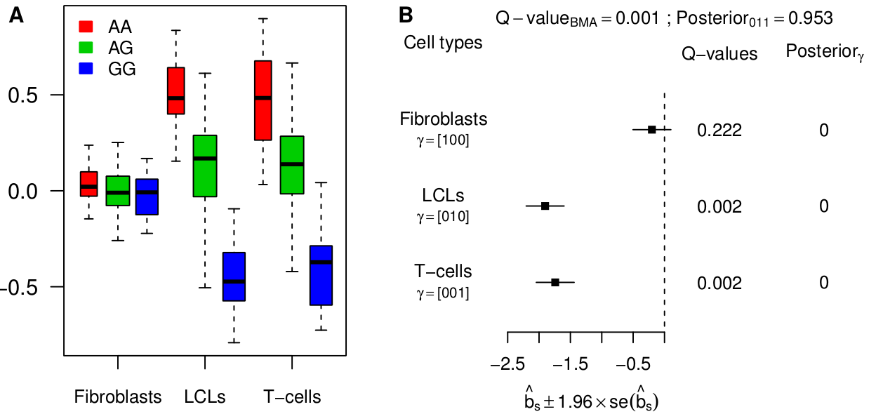
Looking for eQTLs in multiple tissues immediately raises the question of tissue specificity. In this paper, we define an eQTL as “active” in a particular tissue if it has a non-zero genetic effect on the expression of the target gene in this tissue. Most published works implicitly use this definition to refer to tissue-specific eQTLs. One could take issue with this definition: for example, if an eQTL is very strong in one tissue and very weak in another then one might think of this as “tissue-specific”, or at least “tissue-inconsistent”, but in our paper we stick with the binary representation of activity as a useful first step. We represent the activity pattern of a potential eQTL by a binary vector called a configuration (see Han & Eskin, PLoS Genetics 2012, and Wen & Stephens, arXiv 1111.1210). As an example, the following configuration, (110), corresponds to the case where three tissues are analyzed and the eQTL is active only in the first two tissues.
In a brief summary, we can highlight three important features of our model. First, by mapping eQTLs jointly rather than in each tissue separately, our model borrows information between the tissues in which an eQTL is active, and thereby greatly increases power. This is somewhat equivalent to relaxing the threshold of significance in the second tissue when one has already detected the eQTL in the first tissue. Second, by comparing evidence in the data for each configuration, our model provides an interpretation of how an eQTL acts in multiple tissues. In statistical terms, as more than two hypotheses are being tested (for three tissues there are 7 non-null configurations), one usually speaks of model comparison. Third, our model also estimates the proportion of each configuration in the data set. This is achieved by pooling all genes together, and thus borrowing information between them.
Besides simulations, we re-analyzed the largest available data set so far, 3 tissues from 75 individuals, from Dimas et al (Science 2009). Our joint analysis model has more power and detects substantially more eQTLs than a tissue-by-tissue analysis (63% at FDR=0.05). Moreover, we show how a tissue-by-tissue analysis can largely overestimate the fraction of tissue-specific eQTLs, because it does not account for incomplete power when testing in each tissue separately. Qualitatively, the discrepancy between both methods is very large on this data set. Indeed, according to the tissue-by-tissue analysis, only 19% of eQTLs are consistent across tissues, i.e. configuration (111), whereas our model estimates >80% of eQTLs to be consistent. After checking several of our assumptions, we are fairly confident in our estimate. Moreover such a high proportion of consistent eQTLs is also obtained with the pairwise approach originally used by Nica et al (2011).
The analysis of this specific data set therefore indicates that most eQTLs are consistent across tissues. Yet we find examples of strong tissue-specific eQTLs, such as between gene ENSG00000166839 (ANKDD1A) and SNP rs1628955:
Our lab has recently begun to post research pre-prints on arXiv. All members of the group enthusiastically support this trend, both within our own group and within the broader scientific community. The merits of sharing pre-prints have been described elsewhere. The benefits of pre-prints are so immediately apparent, I feel, that there is no need to add further verses to the praises that have already been sung.
Recently, however, my research group and I faced an unusual and difficult question: whether we should post a pre-print that does not describe primary research, but rather is a critique of a recent paper published by another group – a paper on the role of epistasis in molecular evolution from the group led by Fyodor Kondrashov. My group and I have never before written such a commentary; and so I faced this choice with some uncertainty. Here are some thoughts on our group’s decision to write the commentary and to post it to arXiv.
Kondrashov’s group is at the vanguard of contemporary research in molecular evolution. In this particular paper from his group, Breen et al. contend that epistasis is “pervasive throughout protein evolution”; a view that I mostly support and indeed have expressed, in a more limited scope, in several publications and commentaries (e.g. here, here, and here). However, in discussing the paper by Breen et al. over lunch, our research group came to the consensus that their argument is logically flawed. Breen et al. reached their conclusion because the dN/dS values observed in some genes are much lower than their expectation in the absence of epistasis. But when calculating the expected dN/dS ratio in the absence of epistasis, Breen et al. assumed that all amino acids observed in a protein alignment at any particular position have equal fitness. This assumption is unrealistic because, simply, some amino acids may be more fit than others. When we relaxed this unrealistic assumption, we found that the observed dN/dS values and the observed patterns of amino acid diversity at each site are perfectly consistent with a non-epistatic model of protein evolution, for all the nuclear and chloroplast genes in the Breen et al. dataset (but, interestingly, not for their mitochondrial genes).
In an ideal world, scientific disagreements would be resolved by straightforward transactions based solely on logic and data. But in reality, such disagreements inevitably involve intellectual biases, not to mention personalities, politics, reputations, et cetera. In fact, we (my research group and I) are colleagues and admirers of Kondrashov and his comrades (these twopapers of his are among our favorites). Why risk our collegiality by publishing a critique on arXiv?
The answer is two-fold. First, we are passionate about understanding molecular evolution, both as individuals and within the context of a scientific community – and we believe this exchange will advance that understanding. Second, we have had extensive email correspondences with Fedya about the scientific issues at hand. These correspondences have been completely open and straightforward: we have shared our computer code so that Fedya can reproduce our analyses; and Fedya has agreed with our critique, in principle, although he has some reservations and may appreciate subtleties of his data that we do not. In any case, I feel that the scientific exchange has been honest, and it will hopefully avoid the snark that sometimes accompanies such disagreements, and focus instead on the scientific issues at stake.
I wish to thank Graham Coop for inviting me to contribute to Haldane’s Sieve. And thanks of course to my co-authors, including our own fearless leader, David McCandlish.
—Joshua B. Plotkin
N.B.: This blog post is meant as an exchange among scientific colleagues, and not as an advertisement to the media.