
This guest post is by Greg Cooper, Martin Kircher, Daniela Witten, and Jay Shendure, and is a comment on Probabilities of Fitness Consequences for Point Mutations Across the Human Genome by Gulko et al.
Abstract
Recently, Gulko et al. (2014) described an approach, FitCons, to estimate fitness consequences for point mutations using a combination of functional genomic annotations and inferences of selection based on human variant frequency spectra. On the basis of comparisons with several maps of regulatory element features, they concluded that FitCons is substantially better at inferring deleterious regulatory effects of variants than other metrics, including an annotation we developed named Combined Annotation Dependent Depletion (CADD, Kircher et al. 2014). However, we believe that the comparisons of FitCons and CADD for detecting deleterious regulatory variation are misleading, and that methods to predict fitness effects of point mutations should evaluate variants with demonstrable effects rather than variants assumed to have an effect by virtue of being within a functional element. We find that FitCons is substantially less effective than CADD at separating variants, both coding and regulatory, with functional and/or phenotypic effects from functionally inert and/or organismally benign variants. For example, CADD is much more effective at enriching for mutations in two enhancers and one promoter that have been experimentally shown to have large transcriptional effects. Further, in contrast with CADD, FitCons does not separate highly deleterious variants that cause Mendelian disease from high-frequency benign variants, nor does it separate complex-trait associated variants, which are enriched for deleterious regulatory effects, from matched control variants. We believe that it would be more appropriate to characterize FitCons as a predictor of cell-type specific regulatory elements, and to compare it to other tools directed specifically at this task, rather than variant fitness consequences.
Main text
FitCons, recently developed by Gulko et al (2014), is a method to estimate fitness effects of point mutations at both coding and non-coding positions in human genomes. FitCons works by first defining regional boundaries on the basis of clusters of functional genomic signals (“fingerprints”) and then estimating selective effects, inferred from allele frequency distributions within human populations, for variants with the same fingerprint. On the basis of comparisons with enhancers, transcription factor binding sites (TFBSs), and expression quantitative trait loci (eQTLs), Gulko et al. concluded that FitCons is substantially better at inferring variant regulatory effects than other metrics, including an annotation we developed named Combined Annotation Dependent Depletion (CADD, Kircher et al. 2014).
While FitCons is an interesting approach with potentially useful attributes, we believe that the comparisons of FitCons and CADD for detecting deleterious regulatory variation are misleading. Clarification is needed as to the purposes and performances of these metrics. Below, we first describe what we believe to be important general distinctions between CADD and FitCons and then detail their relative effectiveness at differentiating several sets of functional and/or pathogenic variants from inert and/or benign variants. Finally, we consider how correlations between the bin definitions and validation datasets used in Gulko et al., rather than fitness per se, may underlie the performance of FitCons for cell-type specific regulatory element prediction.
CADD is an allele-specific measure of variant deleteriousness that accounts for a wide variety of discrete and quantitative information at the allelic, site, and regional levels (Kircher et al. 2014). CADD scores can vary among the possible alleles at a given site, across sites within a given region or functional element, and between and across variants within differing classes of functional elements. FitCons, on the other hand is driven by a small number of cell-type-specific, regional features with reduced or absent variation within regions. As a result, FitCons is in practice a segmentation method: the median length of uniformly scored segments is 72 bases, the average segment length is 196 bases, and 50% of all scored bases in hg19 lie within a segment over 950 bases long. Furthermore, 30% of all bases in hg19 are assigned to the mode value (0.062), 60% are assigned one of two FitCons values, and over 80% are assigned one of 10 possible values. Thus, FitCons is in practice a regional annotation of cell-type-specific molecular activity, not a site or allele-specific metric of variant deleteriousness.
The basic structures of FitCons and CADD are crucial to interpreting the data presented by Gulko et al. In particular, they measure utility by assessing coverage of bases within functional elements, namely TFBSs and enhancers, relative to genomic background. While such an approach is reasonable to evaluate a method to annotate functional elements, it is not informative for a method to estimate organismal deleteriousness since many mutations within functional elements are evolutionarily neutral, including many that lack even a molecular effect. To wit, by FitCons/INSIGHT estimates, most sites within the enhancers and TFBSs evaluated have fitness effect probabilities below 0.2 (Gulko et al. 2014). While likely somewhat higher among high-information TF-binding motif positions and lower among the enhancers used (mean size of 888 bp), a decisive majority of positions in these nucleotide groups are mutable without consequence. Performance evaluations that reward uniformly high coverage of bases in these regions, rather than the particular subset of variants therein that actually have deleterious molecular effects, are therefore not meaningful for estimates of point mutation fitness consequences.
We firmly believe that methods to predict functional or fitness effects of mutations should be evaluated on mutations for which we have data relevant to function and fitness, not large aggregates of genomic regions or bases within which mutations are simply assumed to be phenotypically relevant. When tested on such mutation sets, we find that FitCons fails to capture a considerable amount of site- and allele-specific information that is captured by CADD (and between-species conservation metrics to a lesser extent). This loss of information, in turn, has profound effects on FitCons’ ability to identify variants with functional, pathogenic, or deleterious effects, including for regulatory changes.
First, FitCons has no predictive power for separating pathogenic variants in ClinVar (Landrum et al. 2014) from benign, high-frequency polymorphisms matched for genic effect category (e.g., missense, nonsense, etc): the distributions of FitCons scores for pathogenic and benign variants are nearly identical (Figure 1). While most of these variants are protein-altering, this same pattern holds for the subset of pathogenic/benign variants that do not directly alter proteins (Figure 1, right). In contrast, CADD and conservation measures like GERP (Cooper et al. 2005) strongly differentiate pathogenic from high-frequency variants, and, although more weakly, also differentiate non-protein-altering pathogenic from benign variants (for further details, see Kircher et al. 2014). The inability of FitCons to distinguish these highly pathogenic/deleterious variants from clearly benign variants runs counter to the general narrative in Gulko et al. in which FitCons scores are claimed to correlate with mutational fitness effect probabilities.

Figure 1. Boxplots showing the score distributions for CADD (top), FitCons (middle), and GERP (bottom), for pathogenic SNVs (red) vs. benign, high-frequency SNVs (blue) chosen to match one-to-one the genic consequence profile of the pathogenic variants. Score distributions for all SNVs are plotted on the left, while the subset of SNVs that are not missense, canonical splice, or nonsense (i.e., “non-protein-altering”) are on the right.
Second, as Gulko et al. emphasize the detection of regulatory variation (title of the manuscript not withstanding), we performed a detailed examination of three regulatory elements for which saturation mutagenesis data exist (Patwardhan et al. 2009; 2012). While not global, these data are comprised of directly measured, not assumed, regulatory effects.
In the 70-bp promoter region of HBB (Patwardhan et al. 2009), FitCons assigns all bases to the genome-wide mode (0.062). However, mutations in this region exhibit substantial variation in both transcriptional and disease consequences. Mutational effects on in vitro promoter activity range from no effect to a >2-fold change in transcription, and some of the strong in vitro effect mutations cause beta-thalassemia by disrupting normal transcript regulation. CADD and GERP correlate significantly with the regulatory (CADD Spearman’s rho=0.23, GERP rho=0.11) and disease consequences of these mutations (details in Kircher et al. 2014).
Within each of two enhancers tested by saturation mutagenesis (Patwardhan et al. 2012), FitCons scores are correlated with mutational effect (ECR11 rho=0.32, ALDOB rho=0.26) similar in magnitude to CADD (ECR11 rho=0.25, ALDOB rho=0.36). However, in both elements, the FitCons correlation is due to a higher score segment overlapping a more transcriptionally active region (Figure 2); no predictive power within the active regions exists. For example, most of the mutations with regulatory effects in the ECR11 enhancer reside in the last ~100 bases, which in turn reside within a single 168-bp FitCons segment. Within this segment, considerable mutational effect variation exists: 209 of 504 possible SNVs, distributed across 110 of the 168 sites, have no discernible effect on transcription (p >= 0.1). Concordantly, these inert mutations have significantly lower CADD scores (Wilcox test p=5.9 x 10⁻²⁵) than their interdigitated SNV neighbors with at least some evidence for functional effect. Furthermore, within the set of mutations that have at least some evidence for effect (p<0.1; other arbitrary thresholds yield similar results), transcriptional effect sizes vary considerably and correlate with CADD (rho=0.33).

Figure 2. Transcriptional effects of individual mutations (log-fold change, y-axis on the left) are plotted (black) against genomic position (hg19, chromosome 2, x-axis). FitCons scores are plotted along the same region in red (y-axis on the right). Within this region there are three FitCons segments, with a segment spanning the last ~168 bases harboring the most active region.
Next, as suggested by Gulko et al., we quantified coverage of discretely thresholded regulatory variants to evaluate the extent to which FitCons and CADD could enrich for “large-effect” regulatory mutations. Specifically, there are 108 mutations that alter transcriptional activity by at least two-fold within the three elements tested (29 mutations across 19 bases in ECR11, 76 mutations across 41 bases in ALDOB, and 3 mutations across 3 sites in HBB). We compared coverage of these 108 mutations at various thresholds relative to coverage of hg19, and find that CADD is much more effective at enriching for them than is FitCons (Figure 3). For example, 95 (88%) of the large-effect regulatory variants have a scaled CADD score above 10, a threshold that includes 10% of all possible hg19 SNVs (~9-fold enrichment above genomic background). Enrichment peaks at a CADD score of 15, a threshold that includes 53.7% of large-effect regulatory variants but only 3.2% of hg19 SNVs (~17-fold enrichment). In contrast, FitCons enrichment peaks at a threshold of 0.08, wherein only ~27% of all large-effect mutations are covered (~4-fold enrichment above background).
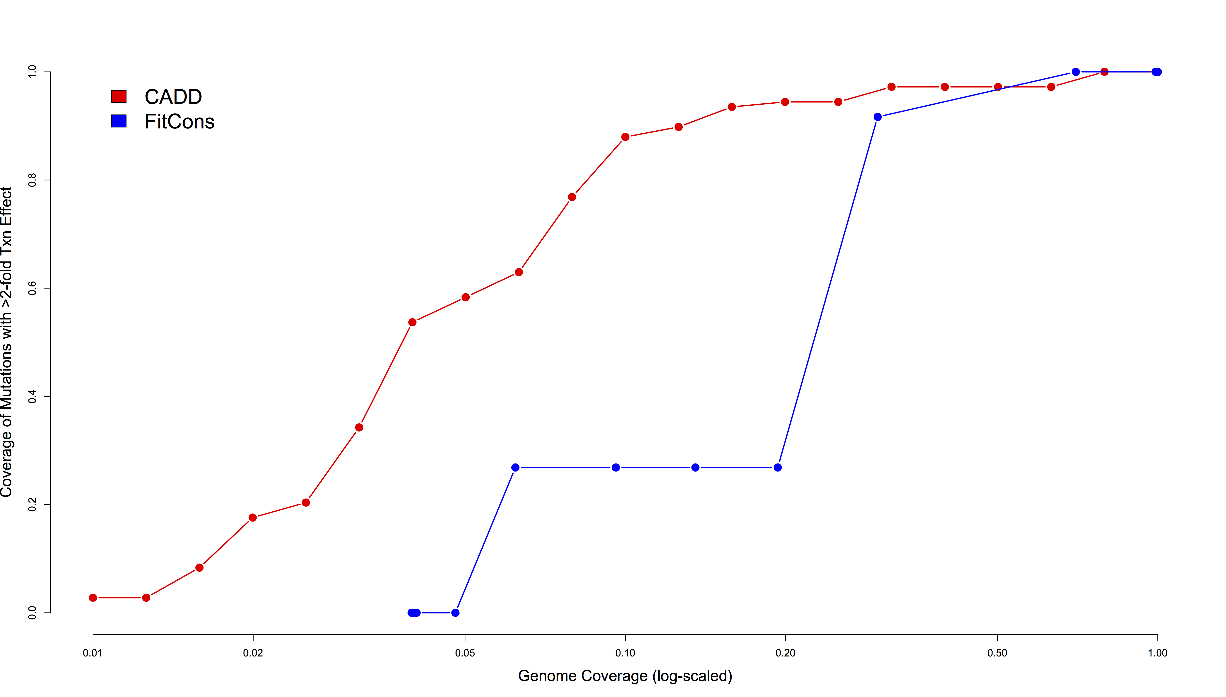
Figure 3. Comparison of coverage levels of large-effect regulatory mutations (y-axis) in two enhancers and one promoter relative to genomic background coverage levels (x-axis, log-scaled) for CADD (red) and FitCons (blue).
We next evaluated the ability of FitCons to distinguish trait-associated SNPs identified in genome-wide association studies (GWAS). Such SNPs are as a group enriched for regulatory variants with pathogenic, likely deleterious effects, a hypothesis supported by numerous anecdotal and systematic studies (e.g., Hindorff et al. 2009; Musunuru et al. 2010; Nicolae et al. 2010; ENCODE Project Consortium et al. 2012). These variants are overwhelmingly non-protein-altering (98%), with ~83% being intronic or intergenic SNPs not near to an exon. We previously showed that CADD scores significantly separate lead GWAS SNPs from matched neighboring control SNPs (Wilcoxon p=5.3 x 10⁻¹²). This separation remains highly significant for the 83% that are intronic or intergenic (p=1.26 x 10⁻⁹), indicating it is not driven solely by coding or near-coding variation. In contrast, FitCons scores do not separate lead GWAS SNPs from controls, either considering all variants (p=0.32) or intronic/intergenic only (p=0.57).
With respect to separation of eQTL SNPs from controls, Gulko et al. used all common variants that were part of the study as a background/control set. We believe the results from such a test are difficult to interpret. They do not control for effects of minor allele frequency, for example, a key property that correlates with both technical (e.g., eQTL discovery power) and biological effects (e.g., eQTL deleteriousness). Additionally, they do not control for genomic location. By virtue of the annotations it uses, FitCons scores will tend to be higher near transcribed genes in the cell-type of choice, which are in turn the only genes for which eQTLs can be identified. Therefore, this analysis confounds the information content resulting from a focus on cis, rather than trans, eQTLs, with that intrinsic to the scores themselves. While this may be an advantage, relative to a more general predictor like CADD, for predicting cell-type-specific function, it likely comes at a cost of reduced accuracy in terms of predicting deleteriousness per se (see below). Furthermore, in practical terms it is not likely to be useful given that cis-effects are the first and major focus of most eQTL discovery efforts, and it is furthermore unclear that FitCons would outperform other cell-type specific regulatory element annotations, such as those from integrative predictions of enhancers and promoters (Ernst and Kellis 2012; Hoffman et al. 2012). In any case, an analysis in which eQTL SNPs are matched for MAF, genomic location, distance to TSS and other confounders would provide a more meaningful evaluation of the utility of FitCons in a realistic eQTL discovery/fine-mapping analysis.
Finally, we believe that the discrepancies in performance metrics defined here vs. within Gulko et al. are also influenced by the potential circularity of cell-type-specific information within both the model definition and validation. Indeed, while INSIGHT adds value by scoring the 624 potential feature-defined bins, the correlations between the bin definitions (expression, DNase, and ChromHMM states) and validation data (TFBSs, enhancers, eQTL candidates) are quite likely the primary drivers of performance of FitCons as measured in Gulko et al. In fact, the strong correlation between INSIGHT and PhyloP as a bin scoring method suggests that metrics of evolutionary constraint could replace INSIGHT in the FitCons framework.
More generally, the use of cell-type specific features in both the metric definition and validation obscures a crucial trade-off in analyses of this sort. Evolutionary constraint-driven metrics (including CADD, which is strongly influenced by evolutionary constraint) emphasize variant effects on organismal fitness, which often have nothing to do with molecular function in any given cell-type; this means that constraint-driven metrics may be sub-optimal when trying to predict molecular function within said cell-type. However, the converse is also true, in that efforts to predict deleteriousness that emphasize cell-type specific molecular functionality will often be misleading when a variant has no molecular effect in that cell-type but strong fitness consequences due to functional effects elsewhere and/or has a molecular effect with no fitness consequence. Obviously, optimal choices in this trade-off depends greatly on analytical context and goals, but in our opinion the goal of predicting “fitness consequences for point mutations” dictates that performance metrics focused on organismal deleteriousness are more appropriate.
As a final illustrative example, Weedon et al. (2014) identified a set of noncoding SNVs that disrupt the function of an enhancer of PTF1A and cause pancreatic agenesis. CADD scores these variants between 23.2 and 24.5, higher than 99.5% of all possible hg19 SNVs and higher than 56% of pathogenic SNVs in ClinVar (most of which are protein-altering); much of the CADD signal for these variants results from measures of mammalian constraint (not shown). FitCons, on the other hand, places these variants in a 5-kb block of sites all scored at the genome-wide mode (0.062). This is in part a result of not having functional genomic data from cells in which the enhancer is active; however, the absence of such data in disease studies is common given that the relevant cell-types are frequently unknown or inaccessible. Further, even if DNase, RNA, and ChromHMM data were all generated for this cell type, given the general distributions of FitCons scores within regulatory elements observed in other cell types and lack of inter-species conservation information, it is unlikely that FitCons would have ranked these variants within the top 0.5% of all possible SNVs.
In any case, Gulko et al. demonstrate that FitCons is reasonably effective, and more so than CADD, at predicting the approximate boundaries of regulatory elements in cell types on which it is trained. However, claims that it better predicts functional or fitness effects of variants in either coding or non-coding regions are unsupported. Indeed, when challenged to separate point mutations with demonstrable effects from appropriate sets of control SNVs, CADD and other metrics that include evolutionary constraint information are substantially better as predictors of both coding and non-coding variant impact. We suggest that it would be more appropriate to characterize FitCons as a predictor of cell-type specific regulatory elements rather than variant fitness consequences, and to compare it to other tools directed at this task, such as ChromHMM (Ernst and Kellis 2012) or Segway (Hoffman et al. 2012).
Acknowledgments
We wish to thank Brad Gulko and Adam Siepel for readily sharing data and engaging in productive dialogue.
References
Cooper GM, Stone EA, Asimenos G, Green ED, Batzoglou S, Sidow A. 2005. Distribution and intensity of constraint in mammalian genomic sequence. Genome Res 15: 901–913.
ENCODE Project Consortium, ENCODE Project Consortium, Dunham I, Dunham I, Kundaje A, Kundaje A, Aldred SF, Aldred SF, Collins PJ, Collins PJ, et al. 2012. An integrated encyclopedia of DNA elements in the human genome. Nature 489: 57–74.
Ernst J, Kellis M. 2012. ChromHMM: automating chromatin-state discovery and characterization. Nat Methods 9: 215–216.
Gulko, B., Hubisz, M.J., Gronau, I., and Siepel, A. 2014. Probabilities of fitness consequences for point mutations across the human genome. bioRxiv. http://dx.doi.org/10.1101/006825
Hindorff LA, Sethupathy P, Junkins HA, Ramos EM, Mehta JP, Collins FS, Manolio TA. 2009. Potential etiologic and functional implications of genome-wide association loci for human diseases and traits. Proc Natl Acad Sci U S A 106: 9362–9367.
Hoffman MM, Buske OJ, Wang J, Weng Z, Bilmes JA, Noble WS. 2012. Unsupervised pattern discovery in human chromatin structure through genomic segmentation. Nat Methods 9: 473–476.
Kircher M, Witten DM, Jain P, O’Roak BJ, Cooper GM, Shendure J. 2014. A general framework for estimating the relative pathogenicity of human genetic variants. Nat Genet 46: 310–315.
Landrum MJ, Lee JM, Riley GR, Jang W, Rubinstein WS, Church DM, Maglott DR. 2014. ClinVar: public archive of relationships among sequence variation and human phenotype. Nucleic Acids Res 42: D980–D985.
Musunuru K, Strong A, Frank-Kamenetsky M, Lee NE, Ahfeldt T, Sachs KV, Li X, Li H, Kuperwasser N, Ruda VM, et al. 2010. From noncoding variant to phenotype via SORT1 at the 1p13 cholesterol locus. Nature 466: 714–719.
Nicolae DL, Gamazon E, Zhang W, Duan S, Dolan ME, Cox NJ. 2010. Trait-associated SNPs are more likely to be eQTLs: annotation to enhance discovery from GWAS. PLoS Genet 6: e1000888.
Patwardhan RP, Hiatt JB, Witten DM, Kim MJ, Smith RP, May D, Lee C, Andrie JM, Lee S-I, Cooper GM, et al. 2012. Massively parallel functional dissection of mammalian enhancers in vivo. Nat Biotechnol 30: 265–270.
Patwardhan RP, Lee C, Litvin O, Young DL, Pe apos er D, Shendure J. 2009. High-resolution analysis of DNA regulatory elements by synthetic saturation mutagenesis. Nat Biotechnol 27: 1173–1175.
Weedon MN, Cebola I, Patch A-M, Flanagan SE, De Franco E, Caswell R, Rodríguez-Seguí SA, Shaw-Smith C, Cho CH-H, Allen HL, et al. 2014. Recessive mutations in a distal PTF1A enhancer cause isolated pancreatic agenesis. Nat Genet 46: 61–64.


